

Classical Mechanics by Konstantin K. Likharev - HTML preview
Download the book in PDF, ePub, Kindle for a complete version.
with
2
F d r.
(7.134)
x
2
t
xz
z
A
Now, if Eq. (129) is satisfied, we again may use the static local relations (75)-(77), with all derivatives d/ dz duly replaced with their partial form / z, to express the force Fx via the bending deformation qx.
Plugging these relations into each other one by one, we arrive at a rather unusual differential equation 41 For this reason, the tensile waves can be called longitudinal only in a limited sense: while the stress wave is purely longitudinal: xx = yy = 0, the strain wave is not: sxx = syy = – szz 0, i.e. q(r, t) n zqz.
Chapter 7
Page 32 of 38
CM: Classical Mechanics
2
4
q
q
A
x EI
x .
(7.135)
2
y
4
t
z
Looking for its solution in the form of a sinusoidal wave (108), we get the following dispersion relation:42
Bending
EI
waves:
2
y
4
k .
(7.136)
dispersion
A
relation
This relation means that the bending waves are not acoustic at any frequency, and cannot be characterized by a single velocity that would be valid for all wave numbers k, i.e. for all spatial Fourier components of a waveform. According to our discussion in Sec. 6.3, such strongly dispersive systems cannot pass non-sinusoidal waveforms too far without changing their waveform rather considerably.
This situation changes, however, if the rod is pre-stretched with a tension force T – just as in the discrete 1D model that was analyzed in Sec. 6.3. The calculation of the effect of this force is essentially similar; let us repeat it for the continuous case, for a minute neglecting the bending stress – see Fig. 13.
T ( z dz)
( z dz)
( z)
y
y
- T ( z)
Fig. 7.13. Additional forces in a thin rod
q
q dq
x
x
x
(“string”), due to the background tension T.
z
z dz
Still sticking to the limit of small angles , the additional vertical component d T x of the net force acting on a small rod fragment of length dz is T x( z – dz) – T x( z) = T y( z + dz) – T y( z) T ( y/ z) dz, so Fx/ z = T ( y/ z). With the geometric relation (77) in its partial-derivative form qx/ z = y, this additional term becomes T (2 qx/ z 2) . Now adding it to the right-hand side of Eq. (135), we get the following dispersion relation
2
1
4
2
EI k k .
(7.137)
A
y
T
Since the product A in the denominator of this expression is just the rod’s mass per unit length (which was denoted in Chapter 6), at low k (and hence low frequencies), this expression is reduced to the linear dispersion law, with the velocity given by Eq. (6.43):
1/ 2
T
v
.
(7.138)
A
So Eq. (137) describes a smooth crossover from the “guitar-string” acoustic waves to the highly dispersive bending waves (136).
42 Note that since the “moment of inertia” Iy, defined by Eq. (70), may depend on the bending direction (unless the cross-section is sufficiently symmetric), the dispersion relation (136) may give different results for different directions of the bending wave polarization.
Chapter 7
Page 33 of 38
CM: Classical Mechanics
Now let us consider another type of transverse waves in thin rods – the so-called torsional waves, which are essentially the dynamic propagation of the torsional deformation discussed in Sec. 6.
The easiest way to describe these waves, again within the limits (129), is to write the equation of rotation of a small segment dz of the rod about the z-axis, passing through the “center of mass” of its cross-section, under the difference of torques = n z z applied on its ends – see Fig. 10: 2
z
I
dz
d ,
(7.139)
z
2
z
t
where Iz is the “moment of inertia” defined by Eq. (91), which now, after its multiplication by dz, i.e.
by the mass per unit area, has turned into the genuine moment of inertia of a dz-thick slice of the rod.
Dividing both sides of Eq. (139) by dz, and using the static local relation (84), z = C = C( z/ z), we get the following differential equation
2
2
I
z C
z .
(7.140)
z
2
2
t
z
Just as Eqs. (111), (115), and (132), this equation describes an acoustic (dispersion-free) wave, which propagates with the following frequency-independent velocity
1/ 2
C
Torsional
v
.
(7.141) waves:
I z
velocity
As we have seen in Sec. 6, for rods with axially-symmetric cross-sections, the torsional rigidity C is described by the simple relation (89), C = Iz, so Eq. (141) is reduced to Eq. (116) for the transverse waves in infinite media. The reason for this similarity is straightforward: in a torsional wave, particles oscillate along small arcs (Fig. 14a), so if the rod’s cross-section is round, its surface is stress-free, and does not perturb or modify the motion in any way, and hence does not affect the transverse velocity.
(a)
(b)
Fig. 7.14. Particle trajectories in two
different transverse waves with the same
velocity: (a) torsional waves in a thin
round rod and (b) circularly polarized
waves in an infinite (or very broad)
sample.
This fact raises an interesting issue of the relation between the torsional and circularly polarized waves. Indeed, in Sec. 7, I have not emphasized enough that Eq. (116) is valid for a transverse wave polarized in any direction perpendicular to the wave vector k (in our notation, directed along the z-axis).
In particular, this means that such waves are doubly degenerate: any isotropic elastic continuum can carry simultaneously two non-interacting transverse waves propagating in the same direction with the same velocity (116), with two mutually perpendicular linear polarizations (directions of the vector a), Chapter 7
Page 34 of 38
CM: Classical Mechanics
for example, directed along the x- and y- axes.43 If both waves are sinusoidal (108), with the same frequency, each point of the medium participates in two simultaneous sinusoidal motions within the [ x, y] plane:
q Re
i( kz t)
a e
A cos ,
Ψ
q Re
i( kz t)
a e
A
(7.142)
x
x
x
y
y
y
cos Ψ ,
where kz – t + x, and y – x. Basic geometry tells us that the trajectory of such a motion on the [ x, y] plane is an ellipse (Fig. 15), so such waves are called elliptically polarized. The most important particular cases of such polarization are:
(i) = 0 or : a linearly-polarized wave, with the displacement vector a is directed at angle =
tan-1( Ay/ Ax) to the x-axis; and
(ii) = /2 and Ax = Ay: two possible circularly-polarized waves, with the right or left polarization, respectively.44
Ay
q( t)
qy
Fig. 7.15. The trajectory of a particle in an
0
qx
elliptically polarized transverse wave, within
A
the plane perpendicular to the direction of
x
wave propagation.
Now comparing the trajectories of particles in the torsional wave in a thin round rod (or pipe) and the circularly polarized wave in a broad sample (Fig. 14), we see that, despite the same wave propagation velocity, these transverse waves are rather different. In the former case (Fig. 14a) each particle moves back and forth along an arc, with the arc’s length different for different particles (and vanishing at the rod’s center), so the waves are not plane. On the other hand, in a circularly polarized wave, all particles move along similar, circular trajectories, so such a wave is plane.
To conclude this chapter, let me briefly mention the opposite limit when the size of the body, from whose boundary the waves are completely reflected,45 is much larger than the wavelength. In this case, the waves propagate almost as in an infinite 3D continuum (which was analyzed in Sec. 7), and the most important new effect is the finite number of wave modes in the body. Repeating the 1D analysis at the end of Sec. 6.5, for each dimension of a 3D cuboid of volume V = l 1 l 2 l 3, and taking into account that the numbers kn in each of the three dimensions are independent, we get the following generalization of 43 As was discussed in Sec. 6.3, this is also true in the simple 1D model shown in Fig. 6.4a.
44 The circularly polarized waves play an important role in quantum mechanics, where they may be most naturally quantized, with their elementary excitations (in the case of mechanical waves we are discussing, called phonons) having either positive or negative angular momentum Lz = .
45 For acoustic waves, such a condition is easy to implement. Indeed, from Sec. 7 we already know that the strong inequality of the wave impedances Z is sufficient for such reflection. The numbers in Table 1 show that, for example, the impedance of a longitudinal wave in a typical metal (say, steel) is almost two orders of magnitude higher than that in air, ensuring their virtually full reflection from the surface.
Chapter 7
Page 35 of 38


Essential Graduate Physics
CM: Classical Mechanics
Eq. (6.75) for the number N of different traveling waves with wave vectors within a relatively small volume d 3 k of the wave vector space:
V
1
3D
3
3
3
dN g
density
d k
d k k ,
(7.143)
2
,
1
for
3
V
of modes
where k >>> 1/ l 1,2,3 is the center of this volume, and g is the number of different possible wave modes with the same wave vector k. For the mechanical waves analyzed above, with one longitudinal mode, and two transverse modes with different polarizations, g = 3.
Note that since the derivation of Eqs. (6.75) and (143) does not use other properties of the waves (in particular, their dispersion relations), this mode counting rule is ubiquitous in physics, being valid, in particular, for electromagnetic waves (where g = 2) and quantum “de Broglie waves” (i.e.
wavefunctions), whose degeneracy factor g is usually determined by the particle’s spin.46
7.9. Exercise problems
7.1. Derive Eqs. (16).
Hint: Besides basic calculus and the definition of the cylindrical coordinates, you may like to use Eq. (4.7) with d = ( d)n z.
7.2. A uniform thin sheet of an isotropic elastic material, of
thickness t and area A >> t 2, is compressed by two plane, parallel, broad, rigid surfaces – see the figure on the right. Assuming that there is no t
slippage between the sheet and the surfaces, calculate the relative
compression (- t/ t) as a function of the compressing force. Compare the A
result with that for the tensile stress calculated in Sec. 3.
7.3. Two opposite edges of a thin but wide sheet of an isotropic elastic material are clamped in two rigid, plane, parallel walls that are pulled apart with force F, along the sheet’s length l. Find the relative extension l/ l of the sheet in the direction of the force and its relative compression t/ t in the perpendicular direction, and compare the results with Eqs. (45)-(46) for the tensile stress and with the solution of the previous problem.
t << R
R
7.4. Calculate the radial extension R of a thin, long, round cylindrical pipe due to its rotation with a constant angular velocity about its symmetry
axis (see the figure on the right), in terms of the elastic moduli E and .
7.5.* A static force F is exerted on an inner point of a uniform and isotropic elastic body.
Calculate the spatial distribution of the deformation created by the force, assuming that far from the point of its application and the points we are interested in, the body’s position is kept fixed.
46 See, e.g., EM Secs. 7.8 and QM Sec. 1.7.
Chapter 7
Page 36 of 38


Essential Graduate Physics
CM: Classical Mechanics
y
t
7.6. A long uniform rail with the cross-section shown in the figure
on the right is being bent with the same (small) torque twice: first within the
xz- plane and then within the yz-plane. Assuming that t << l, find the ratio of l x
the bending deformations in these two cases.
l
7.7. Two thin rods of the same length and mass are made of
the same isotropic and elastic material. The cross-section of one of
them is a circle, while the other one is an equilateral triangle – see
the figure on the right. Which of the rods is stiffer for bending
along its length? Quantify the relation. Does the result depend on
the bending plane’s orientation?
7.8. A thin, uniform, initially straight elastic beam is placed on
x
two point supports at the same height – see the figure on the right. .
z
z
0
0
Calculate the support placements that:
a
a
0
z
(i) ensure that the beam ends are horizontal, and
(ii) minimize the largest deflection of the beam from the
g
horizontal baseline.
Hint: For Task (ii), an approximate answer (with an accuracy better than 1%) is acceptable.
7.9. Calculate the largest longitudinal compression force T
T
T
i
( )
that may be withstood by a thin, straight, elastic rod without
buckling (see the figure on the right) for each of the shown cases:
l
(i) the rod’s ends are clamped, and
T
T
ii
( )
(ii) the rod is free to turn about the support points.
7.10. A thin elastic pole with a square cross-section of area A = a a is firmly dug into the ground in the vertical position, sticking out by height h >> a.
(i) What largest compact mass M may be placed straight on the top of a light pole without stability loss?
(ii) In the absence of such an additional mass, how massive a uniform pole may be to retain its stability?
Hint: For Task (ii), you may use the same WKB approximation as in Problem 6.18.
7.11. Calculate the potential energy of a small and slowly changing, but otherwise arbitrary bending deformation of a uniform, initially straight elastic rod. Can the result be used to derive the dispersion relation (136)?
7.12. Calculate the torsional rigidity of a long uniform rod whose cross-section is an ellipse with semi-axes a and b.
7.13. Calculate the potential energy of a small but otherwise arbitrary torsional deformation z( z) of a uniform and straight elastic rod.
Chapter 7
Page 37 of 38


Essential Graduate Physics
CM: Classical Mechanics
d
N
R
7.14. Calculate the spring constant dF/ dl of a F
F
coil made of a uniform elastic wire with a circular cross-
section of diameter d, wound as a dense round spiral of N
>> 1 turns of radius R >> d – see the figure on the right.
l
F
R
7.15. The coil studied in the previous problem is now used as what is sometimes called the torsion spring – see the figure on the right. Find the d
corresponding spring constant d/ d, where is the torque of the external forces F
0
relative to the center of the coil (point 0).
F
7.16. Use Eqs. (99) and (100) to recast Eq. (101b) for the torsional rigidity C of a thin rod into the form given by Eq. (101c).
7.17.* Generalize Eq. (101b) to the case of rods with more than one cross-section’s boundary.
Use the result to calculate the torsional rigidity of a thin round pipe, and compare it with Eq. (91).
7.18. Prove that in a uniform isotropic medium, an arbitrary (not necessarily plane) elastic wave may be decomposed into a longitudinal wave with ql = 0 and a transverse wave with qt = 0, and find the equations satisfied by these functions.
7.19.* Use the wave equations derived in the solution of the previous problem and the semi-quantitative description of the Rayleigh surface waves given in Sec. 7 of the lecture notes, to calculate the structure of the waves and to derive Eq. (127).
7.20.* Calculate the modes and frequencies of free radial oscillations of a sphere of radius R, made of a uniform elastic material.
7.21. A long steel wire has a circular cross-section with a 3-mm diameter and is pre-stretched with a constant force of 10 N. Which of the longitudinal and transverse waves with frequency 1 kHz has the largest group velocity in the wire? Accept the following parameters for the steel (see Table 1): E =
170 GPa, = 0.30, = 7.8 g/cm3.
7.22. Define and calculate the wave impedances for (i) tensile and (ii)
P
torsional waves in a thin rod, that are appropriate in the long-wave limit. Use
the results to calculate the fraction of each wave’s power P reflected from a
firm connection of a long rod with a round cross-section to a similar rod with a twice smaller diameter – see the figure on the right.
P
7.23. Calculate the fundamental frequency of small transverse standing waves on a free uniform thin rod, and the position of displacement nodes in this mode.
Hint: A numerical solution of the final transcendental equation is acceptable.
Chapter 7
Page 38 of 38
CM: Classical Mechanics
Chapter 8. Fluid Mechanics
This chapter describes the basic notions of fluid mechanics, discusses a few core problems of statics and dynamics of ideal and viscous fluids, and gives a very brief review of such a complicated phenomenon as turbulence. In addition, the viscous fluid flow discussion is used as a platform for an elementary introduction to numerical methods of the partial differential equation solution – whose importance extends well beyond this particular field.
8.1. Hydrostatics
The mechanics of fluids (defined as the materials that cannot keep their geometric form on their own, and include both liquids and gases) is both more simple and more complex than that of elastic solids, with the simplifications mostly in statics.1 Indeed, fluids, by definition, cannot resist static shear deformations. There are two ways to express this fact. First, we can formally take the shear modulus , describing this resistance, to equal zero. Then Hooke’s law (7.32) shows that the stress tensor is diagonal:
.
(8.1)
jj'
jj
jj'
Alternatively, the same conclusion may be reached just by looking at the stress tensor definition (7.19) and/or Fig. 7.3, and saying that in the absence of shear stress, the elementary interface dF has to be normal to the area element dA, i.e. parallel to the vector dA.
Moreover, in fluids at equilibrium, all three diagonal elements jj of the stress tensor have to be equal at each point. To prove that, it is sufficient to single out (mentally rather than physically), from a static fluid, a small volume in the shape of a right prism, with mutually perpendicular faces normal to the two directions we are interested in – in Fig. 1, along the x- and y-axes.
dA
dA ( dA cos)
xx
x
xx
cos
y
Fig. 8.1. Proving the pressure isotropy.
x
dA
The prism is in equilibrium if each Cartesian component of the vector of the total force exerted on all its faces equals zero. For the x-component, this balance may be expressed as xxdAx –
( dA)cos = 0. However, from the geometry (Fig. 1), dAx = dA cos, so the above expression yields
= xx. A similar argument for the y-component gives = yy, so xx = yy. Changing the orientation of the prism, we can get such equalities for any pair of diagonal elements of the stress tensor,
jj, so all three of them have to be equal.
1 It is often called hydrostatics because water has always been the most important liquid for the human race and hence for science and engineering.
© K. Likharev
CM: Classical Mechanics
This common diagonal element of the stress matrix is usually denoted as (- P), because in the vast majority of cases, the parameter P, called pressure, is positive. Thus we arrive at the key relation (which was already mentioned in Sec. 7.2):
.
(8.2)
Pressure
jj'
P
jj'
In the absence of bulk forces, pressure should be constant through the volume of fluid, due to the translational symmetry. Let us see how this result is affected by bulk forces. With the simple stress tensor (2), the general condition of equilibrium of a continuous medium, expressed by Eq. (7.25) with the left-hand side equal to zero, becomes
P f 0 ,
(8.3)
j
rj
and may be re-written in the following convenient vector form:
P f 0.
(8.4)
In the simplest case of a heavy fluid with mass density , in a uniform gravity field f = g, the equation of equilibrium becomes,
P g
0,
(8.5)
with only one nonzero component – near the Earth’s surface, the vertical one. If, in addition, the fluid may be considered incompressible, with its density constant,2 this equation may be readily integrated over the vertical coordinate (say, y) to give the so-called Pascal equation:3
P gy
const,
(8.6)
Pascal
equation
where the direction of the y-axis is taken opposite to that of vector g.
Two manifestations of this key equation are well known. The first one is the fact that in interconnected vessels filled with a fluid, its pressure is equal at all points at the same height ( y), regardless of the vessel shape, provided that the fluid is in equilibrium.4 In particular, if a heavy liquid has an open surface, then in equilibrium, it has to be horizontal – at least, not too close to the retaining walls (see Sec. 2).
The second manifestation of Eq. (6) is the buoyant force Fb exerted by a liquid on a (possibly, partly) submerged body, i.e. the vector sum of the elementary pressure forces dF = PdA exerted on all elementary areas dA of the submerged part of the body’s surface – see Fig. 2. According to Eq. (6), with the constant equal to zero (corresponding to zero pressure at the liquid’s surface taken for y = 0, see Fig.
2a), the vertical component of this elementary force is
2 As was discussed in Sec. 7.3 in the context of Table 7.1, this is an excellent approximation, for example, for human-scale experiments with water.
3 The equation, and the SI unit of pressure 1 Pa 1N/m2, are named after Blaise Pascal (1623-1662) who not only pioneered hydrostatics, but also invented the first mechanical calculator, and made several other important contributions to mathematics – and to Christian philosophy!
4 This simple fact opens wide opportunities for the engineering field of hydraulics, in particular enabling a very simple and efficient way to magnify forces, using interconnected hydraulic cylinders of different diameters.
Chapter 8
Page 2 of 30





Essential Graduate Physics
CM: Classical Mechanics
dF dF cos dA
P cos gy
cos dA
gydA .
(8.7)
y
h
where dAh = cos dA is the horizontal footprint (say, dxdz) of the elementary area dA. Now integrating this relation over all the surface, we get the total vertical buoyant force:5
Archimedes
principle
F g
y dA gV ,
b
(8.8)
h
S
where V is the volume of the submerged part of the body’s volume, while is the liquid’s density, so by magnitude, F b equals the weight of the liquid that would fill the submerged volume.
(a)
(b)
y
dF
dA
after
0
a
V
before
b
dA
A
Fig. 8.2. Calculating
g
g
the buoyant force.
This well-known Archimedes principle may be proved even more simply using the following argument: the liquid’s pressure forces, and hence the resulting buoyant force, cannot depend on what is inside the body’s volume. Hence F b would be the same if we filled the volume V in question with a liquid similar to the surrounding one. But in this case, the liquid should be still in equilibrium even if the surface is completely flexible, so both forces acting on its inner part, the buoyant force Fb and the inner liquid’s weight mg = Vg, have to be equal and opposite, thus proving Eq. (8) again.
Despite the simplicity of the Archimedes principle, its erroneous formulations, such as “The buoyant force’s magnitude is equal to the weight of the displaced liquid” [WRONG!] creep from one undergraduate textbook to another, leading to application errors. A typical example is shown in Fig. 2b, where a solid vertical cylinder with the base area A is pressed into a liquid inside a container of comparable size, pushing the liquid’s level up by distance a. The correct answer for the buoyant force, following from Eq. (8), is
F gV
,
(8.9a)
b
gA a b
because the volume V of the submerged part of the cylinder is evidently A( a + b). But the wrong formulation cited above, using the term displaced liquid, would give a different answer: F gV
gAb . [WRONG!]
(8.9b)
b
displaced
(The latter result is correct only asymptotically, in the limit b/ a .) Another frequent error in hydrostatics concerns the angular stability of a freely floating body –
the problem of vital importance for the boat/ship design. It is sometimes claimed that the body is stable 5 The force is vertical, because the horizontal components of the elementary forces dF exerted on opposite elementary areas dA, at the same height y, cancel.
Chapter 8
Page 3 of 30


Essential Graduate Physics
CM: Classical Mechanics
only if the so-called buoyancy center, the effective point of buoyant force application (in Fig, 3, point B),6 is above the center of mass (C) of the floating body. However, as Fig. 3 shows, this is unnecessary; indeed in the shown case, point B remains below point C, even at a small tilt. Still, in this case, the torque created by the pair of forces Fb and mg tries to return the body to the equilibrium position, which is therefore stable. As Fig. 3 shows, the actual condition of the angular stability may be expressed as the requirement for point M (in shipbuilding, called the metacenter of the ship’s hull) to be above the ship’s center of mass C.7
Fb
M
C
B
Fig. 8.3. Angular stability of a
floating body.
g
m
To conclude this section, let me note that the integration of Eq. (4) may be more complex in the case if the bulk forces f depend on position,8 and/or if the fluid is substantially compressible. In the latter case, Eq. (4) has to be solved together with the medium-specific equation of state = ( P) describing its compressibility law – whose example is given by Eq. (7.38) for ideal gases: mN/ V =
mP/ k B T, where m is the mass of one gas molecule.
8.2. Surface tension effects
Besides the bulk (volume-distributed) forces, one more possible source of pressure is surface tension. This effect results from the difference between the potential energy of atomic interactions on the interface between two different fluids and that in their bulks, and thus may be described by an additional potential energy
U A
,
(8.10) Surface
i
tension
where A is the interface area, and is called the surface tension constant – or just the “surface tension”.
For a stable interface of any two fluids, is always positive.9 For surfaces of typical liquids (or their interfaces with air), at room temperature, the surface tension equals a few 10-2 J/m2,10 corresponding to 6 A simple calculation, similar to the one resulting in Eq. (8), but for the total torque rather than the total force, shows that B is just the center of mass of the submerged volume V filled with any uniform material.
7 It is easy (and hence is left for the reader) to prove that a small tilt of the body leads to a small lateral displacement of point B, but does not affect the position of the metacenter M.
8 A simple example of such a problem is given by the fluid equilibrium in a container rotating with a constant angular velocity . If we solve such a problem in a reference frame rotating together with the container, the real bulk forces should be complemented by the centrifugal “force” (4.93), depending on r.
9 Indeed, if the of the interface of certain two fluids is negative, it self-reconfigures to decrease U i, i.e. to increase U i, by increasing the interface area, i.e. fragments the system into a macroscopically uniform solution.
10 For a better feeling of this number, one should remember that 1 J/m2 1 N/m.
Chapter 8
Page 4 of 30
CM: Classical Mechanics
the potential energy U i of a few 10-2 eV per surface molecule – i.e. just a fraction of the full binding (or
“cohesive”) energy of the same liquid, which is typically of the order of 10-1 eV per molecule.
In the absence of other forces, the surface tension makes a liquid drop spherical to minimize its surface area A at a fixed volume. For the analysis of the surface tension effects for more complex geometries, and in the presence of other forces, it is convenient to reduce them to a certain additional effective pressure drop P ef at the interface. To calculate P ef, let us consider the condition of equilibrium of a small part dA of a smooth interface between two fluids (Fig. 2), in the absence of bulk forces.
P 2
P 1
dA dA
R
dA
,
1 2
r
Fig. 8.4. Deriving the Young-Laplace
formula (13).
If the pressures P 1,2 on the two sides of the interface are different, the work of stress forces on fluid 1 at a small virtual displacement r = n r of the interface (where n = dA/ dA is the unit vector normal to the interface) equals11
W dA r P
.
(8.11)
1
P 2
For equilibrium, this work has to be compensated by an equal change of the interface energy, U i =
( dA). Differential geometry tells us that in the linear approximation in r, the relative change of the elementary surface area, corresponding to a fixed solid angle d, may be expressed as
dA r r
,
(8.12)
dA
R
R
1
2
where R 1,2 are the so-called principal radii of the interface curvature.12 Combining Eqs. (10)-(12), we get the following Young-Laplace formula:13
Young-
1
1
Laplace
P P Δ P
.
(8.13)
1
2
ef
formula
R
R
1
2
11 This equality follows from the general relation (7.30), with the stress tensor elements expressed by Eq. (2), but in this simple case of the net stress force dF = ( P 1 – P 2) dA parallel to the interface element vector dA, it may be even more simply obtained just from the definition of work: W = dFr at the virtual displacement r = n r.
12 This general formula may be readily verified for a sphere of radius r (for which R 1 = R 2 = r and dA = r 2 d, so
( dA)/ dA = ( r 2)/ r 2 = 2 r/ r), and for a round cylindrical interface of radius R (for which R 1 = r, R 2 = , and dA =
rd dz, so ( dA)/ dA = r/ r). For more on curvature, see, for example, M. do Camo, Differential Geometry of Curves and Surfaces, 2nd ed., Dover, 2016.
13 This result (not to be confused with Eq. (15), called Young’s equation) was derived in 1806 by Pierre-Simon Laplace (of the Laplace operator/equation fame) on the basis of the first analysis of the surface tension effects by Thomas Young (yes, the same Young who performed the famous two-slit experiment with light!) a year earlier.
Chapter 8
Page 5 of 30




Essential Graduate Physics
CM: Classical Mechanics
In particular, this formula shows that the additional pressure created by surface tension inside a spherical drop of a liquid, of radius R, equals 2/ R, i.e. decreases with R. In contrast, according to Eqs.
(5)-(6), the pressure effects of bulk forces, for example gravity, grow as gR. The comparison of these two pressure components shows that if the drop radius (or more generally, the characteristic linear size of a liquid’s sample) is much larger than the so-called capillary length
1/ 2
2
a
,
(8.14) Capillary
c
g
length
the surface tension may be safely ignored – as will be done in all following sections of this chapter, besides a brief discussion at the end of Sec. 4. For the water surface, or more exactly its interface with air at ambient conditions, 0.073 J/m2, while 1,000 kg/m3, so a c 4 mm.
On the other hand, in very narrow tubes, such as blood capillary vessels with radius a ~ 1 m, i.e. a << a c, the surface tension effects are very important. The key notion for the analysis of these effects is the contact angle c (also called the “wetting angle”) at an equilibrium edge of a liquid wetting a solid – see Fig. 5.
(a)
(b)
lg
lg
gas
gas
liquid
liquid
c
c
sl
sg
sg
Fig. 8.5. Contact angles
for (a) hydrophilic and
solid
sl
solid
(b) hydrophobic surfaces.
According to its definition (10), the constant may be interpreted as a force (per unit length of the interface boundary) directed normally to the boundary, and “trying” to reduce the interface area. As a result, the balance of horizontal components of the three such forces, shown in Fig. 5a, immediately yields the Young’s equation
cos ,
(8.15) Young’s
sl
lg
c
sg
equation
where the indices of the three constants correspond to three possible interfaces between the liquid, solid, and gas. For the so-called hydrophilic surfaces that “like to be wet” by a particular liquid (not necessarily water), meaning that sl < sg, this relation yields cosc > 0, i.e. c < /2 – the situation shown in Fig. 5a. On the other hand, for hydrophobic surfaces with sl > sg, Eq. (15) yields larger contact angles, c > /2 – see Fig. 5b.
Let us use this notion to solve the simplest and perhaps the most practically important problem of this field – find the height h of the fluid column lifted by the surface tension forces in a narrow vertical tube made of a hydrophilic material, assuming its internal surface to be a round cylinder of radius a – see Fig. 6. Inside an incompressible fluid, pressure drops with height according to the Pascal equation (6), so just below the surface, P P 0 – gh, where P 0 is the background (e.g., atmospheric) pressure. This means that at a << h, the pressure variation along the concave surface (called the meniscus) of the liquid is negligible, so according to the Young-Poisson equation (13), the sum (1/ R 1 +
1/ R 2) has to be virtually constant along the surface. Due to the axial symmetry of the problem, this means that the surface has to be a part of a sphere. From the contact angle definition, the radius R of the Chapter 8
Page 6 of 30




Essential Graduate Physics
CM: Classical Mechanics
sphere is equal to a/cosc – see Fig. 6. Plugging this relation into Eq. (3) with P 1 – P 2 = gh, we get the following result for h:
2 cos
gh
c
.
(8.16a)
a
In hindsight, this result might be obtained more directly – by requiring the total weight gV =
g( a 2 h) of the lifted liquid’s column to be equal to the vertical component F cosc of the full surface tension force F = p, acting on the perimeter p = 2 a of the meniscus. Using the definition (11) of the capillary length a c, Eq. (16a) may be represented as the so-called Jurin rule: Jurin
a 2
a 2
rule
h
c
c
cos
;
(8.16b)
a
c
a
according to our initial assumption h >> a, Eq. (16) is only valid for narrow tubes, with radius a << a c.
a
R
h
c
g
P 0
Fig. 8.6. Liquid’s rise in a vertical capillary tube.
This capillary rise is the basic mechanism of lifting water with nutrients from roots to the branches and leaves of plants, so the tallest tree heights correspond to the Jurin rule (16), with cosc 1, and the pore radius a limited from below by a few microns, because of the viscosity effects restricting the fluid discharge – see Sec. 5 below.
8.3. Kinematics
In contrast to the stress tensor, which is frequently very simple – see Eq. (2), the strain tensor is not a very useful notion in fluid mechanics. Indeed, besides a very few situations,14 typical problems of this field involve fluid flow, i.e. a state when the velocity of fluid particles has some nonzero time average. This means that the trajectory of each particle is a long line, and the very notion of its displacement q from the initial position becomes impracticable. However, the particle’s velocity v
dq/ dt remains a very useful notion, especially if it is considered as a function of the observation point r and (generally) time t. In an important class of fluid dynamics problems, the so-called stationary (or
“ steady ” , or “static”) flow, the velocity defined in this way does not depend on time, v = v(r).
14 One of them is sound propagation, where the particle displacements q are typically small, so the results of Sec.
7.7 are applicable. As a reminder, they show that in fluids, with = 0, the transverse sound cannot propagate, while the longitudinal sound can – see Eq. (7.114).
Chapter 8
Page 7 of 30
CM: Classical Mechanics
There is, however, a price to pay for the convenience of this notion: namely, due to the difference between the vectors q and r, the particle’s acceleration a = d 2q/ dt 2 (that participates, in particular, in the 2nd Newton law) cannot be calculated just as the time derivative of the velocity v(r, t).
This fact is evident, for example, for the static flow case, in which the acceleration of individual fluid particles may be very significant even if v(r) does not depend on time – just think about the acceleration of a drop of water flowing over the Niagara Falls’ rim, first accelerating fast and then virtually stopping below, while the water velocity v at every particular point, as measured from a bank-based reference frame, is nearly constant. Thus the primary task of fluid kinematics is to express a via v; let us do this.
Since each Cartesian component vj of the velocity v has to be considered as a function of four independent scalar variables: three Cartesian components rj of the vector r and time t, its full time derivative may be represented as
dv
v
3
v
dr
j
j
j
j'
.
(8.17)
dt
t
j' 1
r dt
j'
Let us apply this general relation to a specific set of infinitesimal changes { dr 1, dr 2, dr 3} that follows a small displacement dq of a certain particle of the fluid: dr = dq = v dt, i.e.
dr v dt .
(8.18)
j
j
In this case, dvj/ dt is the j th component aj of the particle’s acceleration a, so Eq. (17) yields the following key relation of fluid kinematics:
3
v
v
a
j
v
(8.19a)
j
j .
j'
t
j' 1
rj'
Fluid
Using the del operator , this result may be rewritten in the following compact vector form:15
particle’s
acceleration
v
a
(v )v .
(8.19b)
t
This relation already signals the main technical problem of fluid dynamics: many equations involving the particle’s acceleration are nonlinear in velocity, excluding such a powerful tool as the linear superposition principle (which was used so frequently in the previous chapters of this course) from the applicable mathematical arsenal.
One more basic relation of fluid kinematics is the so-called continuity equation, which is essentially just the differential version of the mass conservation law. Let us mark, inside a fluid flow, an arbitrary volume V limited by a stationary (time-independent) surface S. The total mass of the fluid inside the volume may change only due to its flow through the boundary:
dM
d
d 3 r v d 2 r v dA, (8.20a)
n
dt
dt V
S
S
15 Note that the operator relation d/ dt = / t + (v) is applicable to an arbitrary (scalar or vector) function; it is frequently called the convective derivative. (Alternative adjectives, such as “Lagrangian”, “substantial”, or
“Stokes”, are sometimes used for this derivative as well.) The relation has numerous applications well beyond the fluid dynamics – see, e.g., EM Chapter 9 and QM Chapter 1.
Chapter 8
Page 8 of 30
CM: Classical Mechanics
where the elementary area vector dA is defined just as in Sec. 7.2 – see Fig. 7.
v
A
d
S
V
Fig. 8.7. Deriving the continuity equation.
Now using the same divergence theorem that has been used several times in this course,16 the surface integral in Eq. (20a) may be transformed into the integral of (v) over the volume V, so the relation may be rewritten as
3
j d 0
r
,
(8.20b)
t
V
where the vector j v is called either the mass flux density (or the “mass current ” ). Since Eq. (20b) is valid for an arbitrary stationary volume V, the function under the integral has to vanish at any point: Continuity
equation
j 0.
(8.21)
t
Note that similar continuity equations are valid not only for mass but also for other conserved physics quantities (e.g., the electric charge, probability, etc.), with the proper re-definitions of and j.17
8.4. Dynamics: Ideal fluids
Let us start our discussion of fluid dynamics from the simplest case when the stress tensor obeys Eq. (2) even in motion. Physically, this means that the fluid viscosity effects, leading to mechanical energy loss, are negligible. (The conditions of this assumption will be discussed in the next section.) Then the equation of motion of such an ideal fluid (essentially the 2nd Newton law for its unit volume) may be obtained from Eq. (7.25) using the simplifications of its right-hand side, discussed in Sec. 1:
a P f.
(8.22)
Now using the basic kinematic relation (19), we arrive at the following Euler equation:18
Euler
v
equation
v v P f .
(8.23)
t
Generally, this equation has to be solved together with the continuity equation (21) and the equation of state of the particular fluid, = ( P ). However, as we have already discussed, in many 16 If the reader still needs a reminder, see MA Eq. (12.1).
17 See, e.g., EM Sec. 4.1, QM Sec. 1.4, and SM Sec. 5.6.
18 It was derived in 1755 by the same Leonhard Euler whose name has already been (reverently) mentioned several times in this course.
Chapter 8
Page 9 of 30
CM: Classical Mechanics
situations, the compressibility of water and other important liquids is very low and may be ignored, so
may be treated as a given constant. Moreover, in many cases, the bulk forces f are conservative and may be represented as a gradient of a certain potential function u(r) – the potential energy per unit volume: f
u ;
(8.24)
for example, for a uniform, vertical gravity field, u(r) = gy, where y is measured from some (arbitrary) horizontal level. In this case, the right-hand side of Eq. (23) becomes –( P + u). For these cases, it is beneficial to recast the left-hand of that equation as well, using the following well-known identity of vector algebra19
2
v
v v
v v
.
(8.25)
2
As a result, the Euler equation takes the following form:
2
v
v
v v P u
0.
(8.26)
t
2
In a stationary flow, the first term of this equation vanishes. If the second term, describing fluid’s vorticity, is zero as well, then Eq. (26) has the first integral of motion,
Bernoulli
2
P u v const ,
(8.27) equation
2
called the Bernoulli equation.20 Numerous examples of the application of Eq. (27) to simple problems of stationary flow in pipes, both with and without the Earth gravity field, should be well known to the readers from their undergraduate courses, so I hope I can skip their discussion without much harm.
In the general case, an ideal fluid may have vorticity, so Eq. (27) is not always valid. Moreover, due to the absence of viscosity in an ideal fluid, the vorticity, once created, does not decrease along the so-called streamline – the fluid particle’s trajectory, to which the velocity is tangential at every point.21
Mathematically, this fact22 is expressed by the following Kelvin theorem: (v) dA = const along any small contiguous group of streamlines crossing an elementary area dA.23
However, in many important cases, the vorticity is negligible. For example, even if the vorticity exists in some part of the fluid volume (say, induced by local turbulence, see Sec. 6 below), it may decay due to the fluid’s viscosity, to be discussed in Sec. 5, well before it reaches the region of our interest. (If this viscosity is sufficiently small, its effects on the fluid’s flow in the region of interest are 19 It readily follows, for example, from MA Eq. (11.6) with g = f = v.
20 Named after Daniel Bernoulli (1700-1782), not to be confused with Jacob Bernoulli or one of several Johanns of the same famous Bernoulli family, which gave the world so many famous mathematicians and scientists.
21 Perhaps the most spectacular manifestation of the vorticity conservation is the famous toroidal vortex rings (see, e.g., a nice photo and a movie at https://en.wikipedia.org/wiki/Vortex_ring), predicted in 1858 by H. von Helmholtz, and then demonstrated by P. Tait in a series of spectacular experiments with smoke in the air. The persistence of such a ring, once created, is only limited by the fluid’s viscosity – see the next section.
22 This theorem was first formulated (verbally) by Hermann von Helmholtz.
23 Its proof may be found, e.g., in Sec. 8 of L. Landau and E. Lifshitz, Fluid Mechanics, 2nd ed., Butterworth-Heinemann, 1987.
Chapter 8
Page 10 of 30
CM: Classical Mechanics
negligible, i.e. the ideal-fluid approximation is still acceptable.) Another important case is when a solid body of an arbitrary shape is embedded into an ideal fluid whose flow is uniform (meaning, by definition, that v(r, t) = v0 = const) at large distances,24 its vorticity is zero everywhere. Indeed, since
v = 0 at the uniform flow, the vorticity is zero at distant points of any streamline, and according to the Kelvin theorem, should equal zero everywhere.
In such cases, the velocity distribution, as any curl-free vector field, may be represented as a gradient of some effective potential function,
v
.
(8.28)
Such potential flow may be described by a simple differential equation. Indeed, the continuity equation (21) for a steady flow of an incompressible fluid is reduced to v = 0. Plugging Eq. (28) into this relation, we get the scalar Laplace equation,
2
0 ,
(8.29)
which should be solved with appropriate boundary conditions. For example, the fluid flow may be limited by solid bodies, inside which the fluid cannot penetrate. Then the fluid velocity v at the solid body boundaries should not have a normal component; according to Eq. (28), this means
0 .
(8.30)
surfaces
n
On the other hand, if at large distances the fluid flow is known, e.g., uniform, then:
v const,
r
at .
(8.31)
0
As the reader may already know (for example, from a course on electrodynamics25), the Laplace equation (29) is analytically solvable in several simple (symmetric) but important situations. Let us consider, for example, the case of a round cylinder, with radius R, immersed into a flow with the initial velocity v0 perpendicular to the cylinder’s axis (Fig. 8). For this problem, it is natural to use the cylindrical coordinates, with the z-axis coinciding with the cylinder’s axis. In this case, the velocity distribution is obviously independent of z, so we may simplify the general expression of the Laplace operator in cylindrical coordinates26 by taking / z = 0. As a result, Eq. (29) is reduced to27
1
1
2
,
0
at .
R
(8.32)
2
2
The general solution of this equation may be obtained using the variable separation method, similar to that used in Sec. 6.5 – see Eq. (6.67). The result is28
24 This case is very important, because the motion of a solid body, with a constant velocity u, in the otherwise stationary fluid, gives exactly the same problem (with v0 = -u), in a reference frame bound to the body.
25 See, e.g., EM Secs. 2.3-2.8.
26 See, e.g., MA Eq. (10.3).
27 Let me hope that the letter , used here to denote the magnitude of the 2D radius vector = { x, y}, will not be confused with the fluid’s density – which does not participate in this boundary problem.
28 See, e.g., EM Eq. (2.112). Note that the most general solution of Eq. (32) also includes a term proportional to
, but in our geometry, this term should be zero for such a single-valued function as the velocity potential.
Chapter 8
Page 11 of 30
CM: Classical Mechanics
a b ln
n
c
n s
n a b n
(8.33)
0
0
cos
sin
n
n
n
n
,
n 1
where the coefficients an and bn have to be found from the boundary conditions (30) and (31). Choosing the x-axis to be parallel to the vector v0 (Fig. 8a), so x = cos, we may spell out these conditions in the following form:
,
0
at R,
(8.34)
v cos , at R,
(8.35)
0
0
where 0 is an arbitrary constant, which does not affect the velocity distribution and may be taken for zero. The condition (35) is incompatible with any term of the sum (33) except the term with n = 1 (with s 1 = 0 and c 1 a 1 = – v 0), so Eq. (33) is reduced to
c b
1 1
v
cos.
(8.36)
0
Now, plugging this solution into Eq. (34), we get c 1 b 1 = – v 0 R 2, so, finally, 2
R
v
cos.
(8.37a)
0
y
(a)
(b)
2v
r
0
v0
v
0
0
x
2v0
Fig. 8.8. The flow of an ideal, incompressible fluid around a cylinder: (a) equipotential surfaces and (b) streamlines.
Figure 8a shows the surfaces of constant velocity potential given by Eq. (37a). To find the fluid velocity, it is easier to rewrite that result in the Cartesian coordinates x = cos, y = sin: 2
2
R
R
v x 1
v x 1
.
(8.37b)
0
2
0
2
2
x y
Chapter 8
Page 12 of 30
CM: Classical Mechanics
From here, we may readily calculate the Cartesian components of the fluid’s velocity: 29
2
2
2
y x
R
v
v 1
2
x
R
v
0
x
2
2
x y
1
cos 2
,
2
0
2
(8.38)
xy
R
2
2
2
v
v R
v
y
0
y
2 2
x y
sin 2 .
2
0
2
These expressions show that the maximum fluid’s speed is achieved at the transverse diameter’s ends (
= R, = /2), where v = 2 v 0, while at the longitudinal diameter’s ends ( = R, = 0, ), the velocity vanishes – the so-called stagnation points.
Now the pressure distribution may be calculated by plugging Eqs. (38) into the Bernoulli equation (27) with u(r) = 0. The result shows that the pressure reaches its maximum at the stagnation points, while at the ends of the transverse diameter x = 0, where the velocity is largest, it is lower by 2 v 2
0 . Note that the distributions of both the velocity and the pressure are symmetric with respect to the transverse axis x = 0, so the fluid flow does not create any net drag force in its direction. It may be shown that this result, which stems from the conservation of the mechanical energy of an ideal fluid, remains valid for a solid body of arbitrary shape moving inside an infinite volume of an ideal fluid – the so-called D’Alembert paradox. However, if a body moves near an ideal fluid’s surface, its energy may be transformed into that of the surface waves, and the drag becomes possible.
Speaking about the surface waves: the description of such waves in a gravity field30 is one more classical problem of the ideal fluid dynamics.31 Let us consider an open surface of an ideal liquid of density in a uniform gravity field f = g = - gn y – see Fig. 9.
y
q( y ,
0 z, t)
P P 0
k
A
v( y ,
0 z, t)
0
z
A
Fig. 8.9. Small surface wave on a deep
heavy liquid. Dashed lines show particle
trajectories.
(For
clarity,
the
displacement amplitude A is strongly
g
exaggerated.)
If the wave amplitude A is sufficiently small, we may neglect the nonlinear term (v)v A 2 in the Euler equation (23) in comparison with the first term, v/ t, which is linear in A. For a wave with 29 Figure 8b shows the flow streamlines. They may be found by the integration of the obvious equation dy/ dx =
vy( x, y)/ vx( x, y). For our simple problem, this may be done analytically, giving y(1 – R 2/2) = const, where the constant is specific for each streamline.
30 The alternative, historical term “gravity waves” for this phenomenon may nowadays lead to confusion with the relativistic effect of gravity waves – which may propagate in free space.
31 It was solved by Sir George Biddell Airy (1801-19892), of the Airy functions’ fame. (He was also a prominent astronomer and, in particular, established Greenwich as the prime meridian.)
Chapter 8
Page 13 of 30
CM: Classical Mechanics
frequency and wave number k, the particle’s velocity v = dq/ dt is of the order of A, so this approximation is legitimate if 2 A >> k( A)2, i.e. when kA ,
1
(8.39)
i.e. when the wave’s amplitude A is much smaller than its wavelength = 2/ k. Due to this assumption, we may neglect the liquid vorticity effects, and (for an incompressible fluid) again use the Laplace equation (29) for the wave’s analysis. Looking for its solution in the natural form of a sinusoidal wave, uniform in one of the horizontal directions ( x),
i( kz
)
Re
t
( y) e
,
(8.40)
we get a very simple equation
2
d
2
k 0 ,
(8.41)
2
dy
with an exponential solution (properly decaying at y -), = A exp{ ky}, so Eq. (40) becomes
Re ekyei( kz t) eky cos
,
(8.42)
A
A
kz t
where the last form is valid if A is real – which may be always arranged by a proper selection of the origins of z and/or t. Note that the rate k of the wave’s decay in the vertical direction is exactly equal to the wave number of its propagation in the horizontal direction – along the fluid’s surface. Because of that, the trajectories of fluid particles are exactly circular – see Fig. 9. Indeed, using Eqs. (28) and (42) to calculate velocity components,
v ,
0
v
k eky cos
(8.43)
x
y
A
kz t,
v
k
eky sin
z
A
kz t,
y
z
we see that vy and vz, at the same height y, have equal real amplitudes, and are phase-shifted by /2. This result becomes even more clear if we use the velocity definition v = dq/ dt to integrate Eqs. (43) over time to recover the particle displacement law q( t). Due to the strong inequality (39), the integration may be done at fixed y and z:
ky
ky
k
q q e sin kz t
,
q q e cos kz t
,
q
with
.
(8.44)
y
A
z
A
A
A
Note that the phase of oscillations of vz coincides with that of qy. This means, in particular, that at the wave’s “crest”, particles are moving in the direction of the wave’s propagation – see arrows in Fig. 9.
It is remarkable that all this picture follows from the Laplace equation alone! The “only”
remaining feature to calculate is the dispersion law ( k), and for that, we need to combine Eq. (42) with what remains, in our linear approximation, of the Euler equation (23). In this approximation, and with the bulk force potential u = gy, the equation is reduced to
P gy
0 .
(8.45)
t
Chapter 8
Page 14 of 30
CM: Classical Mechanics
This equality means that the function in the parentheses is constant in space; at the surface, and at negligible surface tension, it should be equal to the pressure P 0 above the surface (say, the atmospheric pressure), which we assume to be constant. This means that on the surface, the contributions to P that come from the first and the third terms in Eq. (45) have to compensate for each other. Let us take the average surface position for y = 0; then the surface with waves is described by the relation y( z, t) = qy( y, z, t) – see Fig. 9. Due to the strong relation (39), we can use Eqs. (42) and (44) with y = 0, so the above compensation condition yields
k
sin
.
(8.46)
A
kz t g sin
A
kz t 0
This condition is identically satisfied on the whole surface (and for any A) as soon as Surface
waves’
2
gk ,
(8.47)
dispersion
This equality is the dispersion relation we were looking for. Looking at this very simple result (which includes just one constant, g), note, first of all, that it does not involve the fluid’s density. This is not too surprising, because due to the weak equivalence principle, particle masses always drop out from the solutions of problems involving gravitational forces alone. Second, the dispersion law (47) is strongly nonlinear, and in particular, does not have an acoustic wave limit at all. This means that the surface wave propagation is strongly dispersive, with both the phase velocity u ph / k = g/ and the group velocity u gr d/ dk = g/2 u ph/2 diverging at 0.32
This divergence is an artifact of our assumption of the infinitely deep liquid. A rather straightforward generalization of the above calculations to a layer of a finite thickness h, using the additional boundary condition vy y=- h = 0, yields a more general dispersion relation:33
2
gk tanh kh.
(8.48)
It shows that relatively long waves, with >> h, i.e. with kh << 1, propagate without dispersion (i.e.
have / k = const u), with the following velocity:
u gh1/ 2 .
(8.49)
For the Earth’s oceans, this velocity is rather high, close to 250 m/s (!) for the average ocean depth h 5
km. This result explains, in particular, the very fast propagation of tsunami waves.
In the opposite limit of very short waves (large k), Eq. (47) also does not give a good description of typical experimental data, due to surface tension effects – see Sec. 2 above. Using Eq. (13), it is easy (and hence also left for the reader’s exercise) to show that their account leads (at kh >> 1) to the following modification of Eq. (47):
2
3
k
gk
.
(8.50)
32 Here, unlike in Chapters 6 and 7, the wave velocity is denoted by the letter u to avoid any chance of confusion with the velocity v (43) of the liquid’s particles.
33 This calculation (left for the reader’s exercise), shows also that at finite h, the particle trajectories are elliptical rather than circular, becoming more and more stretched in the wave propagation direction near the bottom of the layer.
Chapter 8
Page 15 of 30
CM: Classical Mechanics
According to this formula, the surface tension is important at wavelengths smaller than the capillary constant a c given by Eq. (14). Much shorter waves, for that Eq. (50) yields k 3/2, are called the capillary waves – or just “ripples”.
8.5. Dynamics: Viscous fluids
The viscosity of many fluids, at not overly high velocities, may be described surprisingly well by adding, to the static stress tensor (2), additional elements proportional to the velocity v dq/ dt:
~
P
(v) .
(8.51)
jj '
jj'
jj'
In view of our experience with Hooke’s law (7.32) expressing a stress tensor proportional to particle displacements q, we may expect a similar expression with the replacement q v = dq/ dt:
1
1
~
2 e
(8.52a)
jj'
Tr
jj'
jj
jj'
'
e 3
Tre ,
3
3
where ejj’ are the elements of the symmetrized strain derivative tensor: ds
1 v
v
e
jj' j
j' .
(8.52b)
jj'
dt
2 r
r
j'
j
Experiment confirms that Eq. (52) gives a good description of the viscosity effects in a broad range of isotropic fluids. The coefficient is called either the shear viscosity, or the dynamic viscosity, or just viscosity, while is called the second (or bulk) viscosity.
In the most frequent case of virtually incompressible fluids, Tr (e) = d[Tr (s)]/ dt = ( dV/ dt)/ V = 0, so the term proportional to vanishes, and is the only important viscosity parameter.34 Table 1 shows the approximate values of the viscosity, together with the mass density , for several representative fluids.
Table 8.1. Important parameters of several representative fluids (approximate values) Fluid (all at 300 K, until indicated otherwise)
(mPas)
(kg/m3)
Glasses
1021–1024
2,200–2,500
Earth magmas (at 800 to 1,400 K)
104–1014
2,200–2,800
Machine oils (SAE 10W – 40 W)
65-320
900
Water
0.89
1,000
Mercury
1.53
13,530
Liquid helium 4 (at 4.2K, 105 Pa)
0.019
130
Air (at 105 Pa)
0.018
1.3
34 Probably the most important effect we miss by neglecting is the attenuation of the (longitudinal) acoustic waves, into which the second viscosity makes a major contribution – whose (rather straightforward) analysis is left for the reader’s exercise.
Chapter 8
Page 16 of 30


Essential Graduate Physics
CM: Classical Mechanics
One can see that may vary in very broad limits; the extreme cases of fluids are glasses (which, somewhat counter-intuitively, are not stable solids even at room temperature, but rather may “flow”, though extremely slowly, until they eventually crystallize) and liquid helium (whose viscosity is of the order of that of gases,35 despite its much higher density).
Incorporating the additional elements of jj’ to the equation (23) of fluid motion, absolutely similar to how it was done at the derivation of Eq. (7.107) of the elasticity theory, and with the account of Eq. (19), we arrive at the famous Navier-Stokes equation:36
Navier-
v
2
Stokes
v v P f v v.
(8.53)
equation
t
3
The apparent simplicity of this equation should not mask a big range of phenomena that are described by it (notably turbulence – see the next section), and the enormous complexity of some solutions even for some simple geometries. In most problems interesting for practice, the only option is to use numerical methods, but due to a large number of parameters (, , , plus geometrical parameters of the involved bodies, plus the distribution of bulk forces f, plus boundary conditions), this way is strongly plagued by the curse of dimensionality that was discussed in the end of Sec. 5.8.
Let us see how the Navier-Stokes equation works, on several simple examples. As the simplest case, let us consider the so-called Couette flow of an incompressible fluid layer between two wide, horizontal plates (Fig. 10), caused by their mutual sliding with a constant relative velocity v0.
v
y
0
d
v( y)
Fig. 8.10. The simplest problem of
the viscous fluid flow.
0
z
Let us assume a laminar (vorticity-free) fluid flow. (As will be discussed in the next section, this assumption is only valid within certain limits.) Then we may use the evident symmetry of the problem, to take, in the coordinate frame shown in Fig. 10, v = nz v( y). Let the bulk forces be vertical, f = n yf, so they do not give an additional drive to the fluid flow. Then for the stationary flow (v/ t = 0), the vertical, y- component of the Navier-Stokes equation is reduced to the static Pascal equation (6), showing that the pressure distribution is not affected by the plate (and fluid) motion. In the horizontal, z-
component of the equation, only one term, 2 v, survives, so for the only Cartesian component of the fluid’s velocity we get the 1D Laplace equation
2
d v
.
0
(8.54)
2
dy
35 Actually, at even lower temperatures (for He 4, at T < T 2.17 K), helium becomes a superfluid, i.e. loses its viscosity completely, as a result of the Bose-Einstein condensation – see, e.g., SM Sec. 3.4.
36 Named after Claude-Louis Navier (1785-1836) who had suggested the equation, and Sir George Gabriel Stokes (1819-1903) who has demonstrated its relevance by solving the equation for several key situations.
Chapter 8
Page 17 of 30
CM: Classical Mechanics
In contrast to the ideal fluid (see, e.g., Fig. 8b), the relative velocity of a viscous fluid and a solid wall it flows by should approach zero at the wall,37 so Eq. (54) should be solved with boundary conditions
,
0
at y ,
0
v
(8.55)
v , at y d.
0
Using the evident solution to this boundary problem, v( y) = ( y/ d) v 0, illustrated by the arrows in Fig. 10, we can now calculate the horizontal drag force acting on a unit area of each plate. For the bottom plate, F
v
v
z
0
.
(8.56)
zy y0
y0
A
y
d
y
(For the top plate, the derivative v/ y has the same value, but the sign of dAy has to be changed to reflect the direction of the outer normal to the solid surface, so we get a similar force but with the negative sign.) The well-known result (56) is often used, in undergraduate physics courses, for a definition of the dynamic viscosity , and indeed shows its meaning very well.38
As the next, slightly less trivial example let us consider the so-called Poiseuille problem:39
finding the relation between the constant external pressure gradient - P/ z applied along a round pipe with internal radius R (Fig. 11) and the so-called discharge Q – defined as the mass of fluid flowing through the pipe’s cross-section in unit time.
higher
R
lower
pressure
v()
pressure
0
z
Fig. 8.11. The Poiseuille problem.
Again assuming a laminar flow, we can involve the problem’s uniformity along the z-axis and its axial symmetry to infer that v = n zv(), and P = - z + f(, ) + const (where = {, } is again the 2D
radius vector rather than the fluid density), so the Navier-Stokes equation (53) for an incompressible fluid (with v = 0) is reduced to the following 2D Poisson equation:
2 v .
(8.57)
2
After spelling out the 2D Laplace operator in polar coordinates for our axially-symmetric case / = 0, Eq. (57) becomes a simple ordinary differential equation,
37 This is essentially an additional experimental fact, which that may be understood as follows. The tangential component of the velocity should be continuous at the interface between two viscous fluids, in order to avoid infinite stress – see Eq. (52), and solid may be considered as an ultimate case of fluid, with infinite viscosity.
38 The very notion of viscosity was introduced (by nobody other than the same Sir Isaac Newton) via a formula similar to Eq. (56), so any effect resulting in a drag force proportional to velocity is frequently called Newtonian viscosity.
39 It was solved by G. Stokes in 1845 to explain the experimental results obtained by Gotthilf Hagen in 1839 and (independently) by Jean Poiseuille in 1840-41.
Chapter 8
Page 18 of 30


Essential Graduate Physics
CM: Classical Mechanics
1 d
dv
(
) ,
(8.58)
d
d
which has to be solved on the segment 0 R, with the following boundary conditions: v ,
0
at R,
dv
(8.59)
,
0
at 0.
d
(The latter condition is required by the axial symmetry.) A straightforward double integration yields:
v
2 2
R ,
(8.60)
4
so the (easy) integration of the mass flow density over the cross-section of the pipe, R
2
Q vd r 2
( 2
2
R ) d ,
(8.61)
4
A
0
immediately gives us the so-called Poiseuille (or “Hagen-Poiseuille”) law for the fluid’s discharge: Poiseuille
law
4
Q
R .
(8.62)
8
The most prominent (and practically important) feature of this result is a very strong dependence of the discharge on the pipe’s radius.
Of course, the 2D Poisson equation (57) is so readily solvable not for each cross-section shape.
For example, consider a very simple, square-shaped cross-section with side a (Fig. 12).
y
a / 2
Fig. 8.12. Application of the finite-difference
a
method with a very coarse mesh (with step h
= a/2) to the problem of viscous fluid flow in
2
a pipe with a square cross-section.
0
x
In this case, it is natural to use the Cartesian coordinates aligned with the cross-section’s sides, so Eq. (57) becomes
2
2
v v
0
for
const,
x, y a,
(8.63)
2
2
x
y
and has to be solved with boundary conditions
v ,
0
at x, y ,
0 a .
(8.64)
For this boundary problem, analytical methods such as the variable separation lead to answers in the form of infinite sums (series), which ultimately require computers anyway – at least for their plotting Chapter 8
Page 19 of 30
CM: Classical Mechanics
and comprehension. Let me use this pretext to discuss how explicitly numerical methods may be used for such problems – or for any partial differential equations involving the Laplace operator. The simplest of them is the finite-difference method40 in which the function to be calculated, f(r), is represented by its values f(r1), f(r2), … in discrete points of a rectangular grid (frequently called mesh) of the corresponding dimensionality – Fig. 13.
(a)
(b)
f
f
f
( f / r )
j
f
/ r
j
f
f
f
f
h
Fig. 8.13. The idea of the finite-
f
difference method in (a) one and
h
(b) two dimensions.
r
h
h
j
In Sec. 5.7, we have already discussed how to use such a grid to approximate the first derivative of the function – see Eq. (5.97). Its extension to the second derivative is straightforward – see Fig. 13a:41
2
f
f
1 f
f
1 f f
f f
f f 2 f
.
(8.65)
2
2
r
r
r
h
r
r
h
h
h
h
j
j
j
j
j
The relative error of this approximation is of the order of h 24 f/ r 4 j, quite acceptable in many cases. As a result, the left-hand side of Eq. (63), treated on a square mesh with step h (Fig. 13b), may be approximated with the so-called five-point scheme:
2
2
v v
v v 2 v
v v 2 v
v v v v 4 v
.
(8.66)
2
2
2
2
2
x
y
h
h
h
(The generalization to the seven- point scheme, appropriate for 3D problems, is straightforward.) Let us apply this scheme to the tube with the square cross-section, using an extremely coarse mesh with step h
= a/2, shown in Fig. 12. In this case, the fluid velocity v should equal zero at the walls, i.e. at all points of the five-point scheme except for the central point (in which the velocity obviously reaches its maximum), so Eqs. (63) and (66) yield42
0 0 0 0 4 v
1 a
max
2
,
i.e. v
(8.67)
2
( a / )
2
max
16
40 For more details see, e.g., R. Leveque, Finite Difference Methods for Ordinary and Partial Differential Equations, SIAM, 2007.
41 As a reminder, at the beginning of Sec. 6.4 we have already discussed the reciprocal transition – from a similar sum to the second derivative in the continuous limit ( h 0).
42 Note that the value (67) of v max is exactly the same as given by the analytical formula (60) for the round cross-section with the radius R = a/2. This is not an occasional coincidence. The velocity distribution given by (60) is a quadratic function of both x and y. For such functions, with all derivatives higher than 2 f/ r 2 j equal to zero, equation (66) is exact rather than approximate.
Chapter 8
Page 20 of 30
Essential Graduate Physics
CM: Classical Mechanics
This result for the maximal velocity is only ~20% different from the exact value. Using a slightly finer mesh with h = a/4, which gives a readily solvable system of three linear equations for three different velocity values (the exercise left for the reader), brings us within just a couple of percent from the exact result. So numerical methods may be practically more efficient than the “analytical” ones, even if the only available tool is a calculator app on your smartphone rather than an advanced computer.
Of course, many practical problems of fluid dynamics do require high-performance computing, especially in conditions of turbulence with its complex, irregular spatial-temporal structure – see the next section). In such cases, the finite-difference approach discussed above may become unsatisfactory, because it implies the same accuracy of the derivative approximation through the whole area of interest.
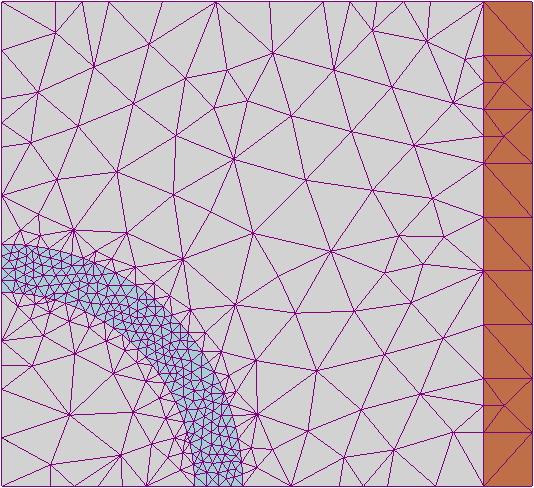
A more powerful (but also much more complex for implementation) approach is the finite-element method in which the discrete-point mesh is based on triangles with unequal sides and is (in most cases, automatically) generated from the system geometry, giving more mesh points at the location(s) of the higher gradients of the calculated function (Fig. 14), and hence a better calculation accuracy for the same total number of points. Unfortunately, I do not have time/space to go into the details of that method, so the interested reader is referred to the special literature on this subject.43
Fig. 8.14. A typical finite-element
mesh generated automatically for a
system with relatively complex
geometry – a round cylindrical shell
inside another one, with mutually
perpendicular axes. (Adapted from
the
original
by
I.
Zureks,
https://commons.wikimedia.org/w/in
dex.php?curid=2358783, under the
CC license BY-SA 3.0.)
Before proceeding to our next topic, let me mention one more important problem that is analytically solvable using the Navier-Stokes equation: a slow motion of a solid sphere of radius R, with a constant velocity v0, through an incompressible viscous fluid – or equivalently, a slow flow of the fluid (uniform at large distances) around an immobile sphere. In the limit v 0, the second term on the left-hand side of Eq. (53) is negligible (just as at the surface wave analysis in Sec. 3), the equation takes the form
2
P v ,
0
for R r ,
(8.68)
and should be complemented with the incompressibility condition v = 0 and the boundary conditions 43 I can recommend, e.g., C. Johnson, Numerical Solution of Partial Differential Equations by the Finite Element Method, Dover, 2009, or T. Hughes, The Finite Element Method, Dover, 2000.
Chapter 8
Page 21 of 30
CM: Classical Mechanics
v
0,
at r R ,
(8.69)
v v , at r .
0
In spherical coordinates, with the polar axis directed along the vector v0, this boundary problem has axial symmetry (so v/ = 0 and v = 0), and allows the following analytical solution:
3
3
R
R
3
3
R
R
3 v R
v v cos 1
,
0
v v
P
.
(8.70)
r
0
2
sin 1
,
cos
2 r
2
0
r
4 r
4 2
r
2 2
r
Now calculating the tensor elements (52b) at r = R, using them to find the stress tensor elements from Eq. (52a), and integrating the elementary forces (7.18) over the surface of the sphere, it is straightforward to obtain the famous Stokes formula for the drag force acting on the sphere:44
F 6 Rv .
(8.71) Stokes
0
formula
For water drops with a 1-micron diameter, usually taken for the border between aerosols and droplets, descending in the ambient-condition air under their own weight, it predicts an equilibrium velocity v of close to 0.1 meters per hour, with the further scaling v R 2.45 (Note, however, that at R below ~10 m, corrections due to air molecule discreteness become noticeable.)
For what follows in the next section, it is convenient to recast this result into the following form: 24
C
,
(8.72)
d
e
R
where C d is the drag coefficient defined as
F
C
,
(8.73)
d
2
v
A/ 2
0
with A R 2 being the sphere’s cross-section “as seen by the incident fluid flow”, and Re is the so-called Reynolds number.46 In the general case, the number is defined as
vl
e
R
,
(8.74) Reynolds
number
where l is the linear-size scale of the problem, and v is its velocity scale. (In the particular case of Eq.
(72) for the sphere, l is identified with the sphere’s diameter D = 2 R, and v with v 0). The physical sense of these two definitions will be discussed in the next section.
44 This formula played an important role in the first precise (better than 1%) calculation of the fundamental electric charge e by R. Millikan and H. Fletcher from their famous oil drop experiments in 1909-1913.
45 These numbers are of key importance not only for the recent heated discussions of contagious disease transmission, but also for many other fields including atmospheric physics. For example, for an average water droplet in clouds, with R ~ 10 m, Eq. (71) (even with a due account of a slightly lower air viscosity at typical cloud heights) yields the descent velocity of the order of 10 m/hr, substantiating the correct answer to the popular high-school question, “Why clouds do not fall?” (The answer is: water droplets do descend, but so slowly that they has ample time to evaporate near the lower surface of the cloud, so the cloud as a whole may maintain its height.)
46 This notion was introduced in 1851 by the same G. Stokes but eventually named after O. Reynolds who popularized it three decades later.
Chapter 8
Page 22 of 30
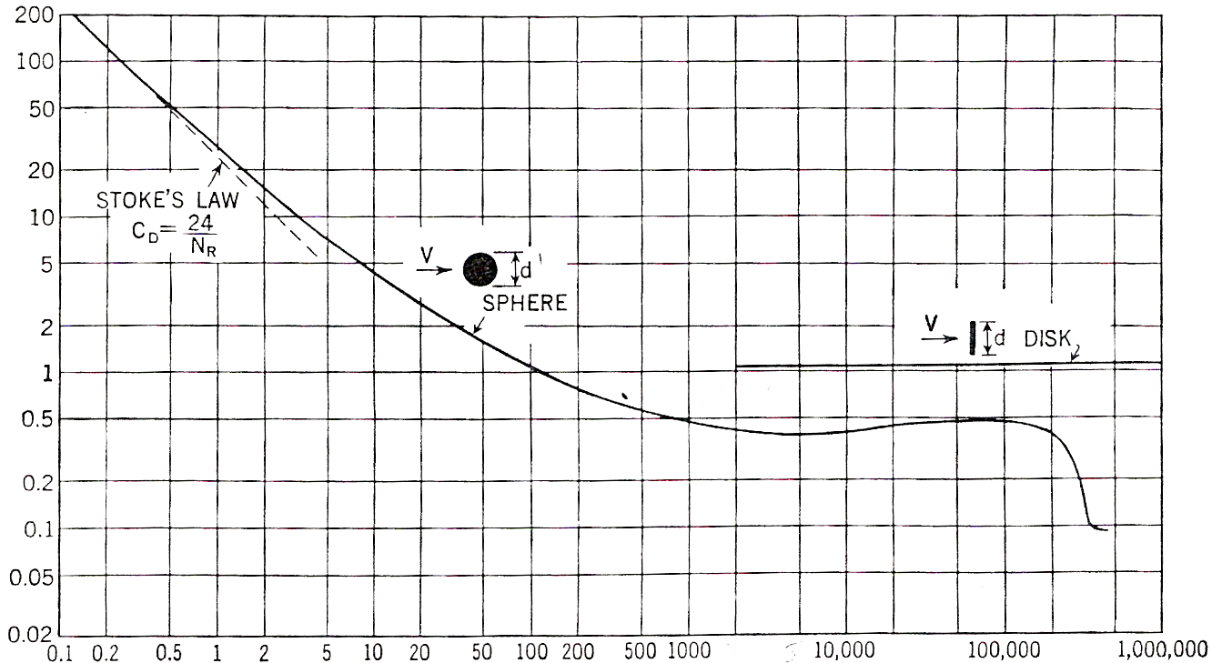
Essential Graduate Physics
CM: Classical Mechanics
8.6. Turbulence
As Fig. 15 shows, the Stokes result (71)-(72) is only valid at Re << 1, while for larger values of the Reynolds number, i.e. at higher velocities v 0, the drag force is larger. This very fact is not quite surprising, because at the derivation of the Stokes’ result, the nonlinear term (v)v in the Navier-Stokes equation (53), which scales as v 2, was neglected in comparison with the linear terms, scaling as v. What is more surprising is that the function C d( Re) exhibits such a complicated behavior over many orders of the velocity’s magnitude, giving a hint that the fluid flow at large Reynolds numbers should be also very complicated. Indeed, the reason for this complexity is a gradual development of very intricate, time-dependent fluid patterns, called turbulence, rich with vortices – for example, see Fig. 16. These vortices are especially pronounced in the region behind the moving body (the so-called wake), while the region before the body remains almost unperturbed. As Fig. 15 indicates, the turbulence exhibits rather different behaviors at various velocities (i.e. values of Re), and sometimes changes rather abruptly – see, for example, the significant drag’s drop at Re 5105.
C d
Re
Fig. 8.15. The drag coefficient for a sphere and a thin round disk as functions of the Reynolds number.
Adapted from F. Eisner, Das Widerstandsproblem, Proc. 3rd Int. Cong. on Appl. Mech., Stockholm, 1931.
In order to understand the conditions of this phenomenon, let us estimate the scale of various terms of the Navier-Stokes equation (53) for a generic body with characteristic size l, moving in an otherwise static incompressible fluid, with velocity v. In this case, the time scale of possible non-stationary phenomena is given by the ratio l/ v,47 so we arrive at the following estimates: 47 The time scale of phenomena in externally-driven systems may be different; for example, for forced oscillations with frequency , it may be the oscillation period T 2/. For such problems, the ratio S ( l/ v)/ T, commonly called either the Strouhal number or the reduced frequency, serves as another dimensionless constant.
Chapter 8
Page 23 of 30
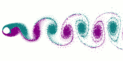
Essential Graduate Physics
CM: Classical Mechanics
v
v
2
v
f
v
Equation term:
t
(8.75)
2
2
v
v
v
g
2
Order of magnitude:
l
l
l
(I have skipped the term P because as we have seen in the previous section, in typical fluid flow problems, it balances the viscosity term, and hence is of the same order of magnitude.) uniform
fluid flow
solid
sphere
Fig. 8.16. A snapshot of the turbulent tail ( wake) behind a sphere moving in a fluid with a high Reynolds number, showing the so-called von Kármán vortex street. Adapted from the original (actually, a very nice animation, http://www.mcef.ep.usp.br/staff/jmeneg/cesareo/vort2.gif) by Cesareo de La Rosa Siqueira, as a copyright-free material, available at https://commons.wikimedia.org/w/index.php?curid=87351.
Estimates (75) show that the relative importance of the terms may be characterized by two dimensionless ratios.48 The first of them is the so-called Froude number 49
2
v
/
2
l
v
F
,
(8.76)
g
lg
which characterizes the relative importance of the gravity – or, upon appropriate modification, of other bulk forces. In most practical problems (with the important exception of surface waves, see Sec. 4
above), F >> 1 so the gravity effects may be neglected.
Much more important is another ratio, the Reynolds number (74), which may be rewritten as 2
vl
v
/ l
e
R
,
(8.77)
2
v / l
and hence is a measure of the relative importance of the fluid particle’s inertia in comparison with the viscosity effects.50 So again, it is natural that for a sphere, the role of the vorticity-creating term (v)v 48 For substantially compressible fluids (e.g., gases), the most important additional dimensionless parameter is the Mach number M v/ v l, where v l = ( K/)1/2 is the velocity of the longitudinal sound – which is, as we already know from Chapter 7, the only wave mode possible in an infinite fluid. Especially significant for practice are supersonic effects (including the shock wave in the form of the famous Mach cone with half-angle M = sin-1 M-1) that arise at M > 1. For a more thorough discussion of these issues, I have to refer the reader to more specialized texts – either Chapter IX of the Landau-Lifshitz volume cited above or Chapter 15 in I. Cohen and P. Kundu,
Fluid Mechanics, 4th ed., Academic Press, 2007 – which is generally a good book on the subject.
49 Named after William Froude (1810-1879), one of the applied hydrodynamics pioneers.
50 Note that the “dynamic” viscosity participates in this number (and many other problems of fluid dynamics) only in the combination /, which thereby has deserved a special name of kinematic viscosity.
Chapter 8
Page 24 of 30
CM: Classical Mechanics
becomes noticeable already at Re ~ 1 – see Fig. 15. What is very counter-intuitive is the onset of turbulence in systems where the laminar (turbulence-free) flow is formally an exact solution to the Navier-Stokes equation for any Re. For example, at Re > Re t 2,100 (with l 2 R and v v max) the laminar flow in a round pipe, described by Eq. (60), becomes unstable, and the resulting turbulence decreases the fluid discharge Q in comparison with the Poiseuille law (62). Even more strikingly, the critical value of Re is rather insensitive to the pipe wall roughness and does not diverge even in the limit of perfectly smooth walls.
Since Re >> 1 in many real-life situations, turbulence is very important for practice. (Indeed, the values of and for water listed in Table 1 imply that even for a few-meter-sized object, such as a human body or a small boat, Re > 1,000 at any speed above just ~1 mm/s.) However, despite nearly a century of intensive research, there is no general, quantitative analytical theory of this phenomenon, and most results are still obtained either by rather approximate analytical treatments, or by the numerical solution of the Navier-Stokes equations using the approaches discussed in the previous section, or in experiments (e.g., on scaled models51 in wind tunnels). A rare exception is the relatively recent theoretical result by S. Orszag (1971) for the turbulence threshold in a flow of an incompressible fluid through a gap of thickness t between two parallel plane walls (see Fig. 10): Re t 5,772 (for l t/2 and v
v max). However, even for this simplest geometry, the analytical theory still cannot predict the turbulence patterns at Re > Re t. Only certain general, semi-quantitative features of turbulence may be understood from simple arguments.
For example, Fig. 15 shows that within a very broad range of Reynolds numbers, from ~102 to
~3105, C d of a thin round disk perpendicular to the incident flow, C d is very close to 1.1 for any Re > 103, and that of a sphere is not too far away. The approximate equality C d 1, meaning that the drag force F is close to v 2
0 A/2, may be understood (in the picture where the object is moved by an external force F with the velocity v 0 through a fluid that was initially at rest) as the equality of the force-delivered power Fv
2
0 and the fluid’s kinetic energy ( v 0 /2) V created in volume V = v 0 A in unit time. This relation would be exact if the object gave its velocity v 0 to each and every fluid particle its cross-section runs into, for example by dragging all such particles behind itself. In reality, much of this kinetic energy goes into vortices, where the particle velocity may differ from v 0, so the equality C d 1 is only approximate.
Another important general effect is that at very high values of Re, fluid flow at the leading surface of solid objects forms a thin, highly turbulent boundary layer that matches the zero relative velocity of the fluid at the surface with its substantial velocity in the outer region, which is almost free of turbulence and many cases, of other viscosity effects. This fact, clearly visible in Fig. 16, enables semi-quantitative analyses of several effects, for example, the so-called Magnus lift force 52 Fl exerted (on top of the usual drag force Fd) on rotating objects, and directed across the fluid flow – see Fig. 17.
An even more important application of this concept is an approximate analysis of the forces exerted on non-rotating airfoils (such as aircraft wings) with special cross-sections forming sharp angles at their back ends. Such a shape minimizes the airfoil’s contacts with the vortex street it creates in its 51 The crucial condition of correct modeling is the equality of the Reynolds numbers (74) (and if relevant, also of the Froude numbers and/or the Mach numbers) of the object of interest and its model.
52 Named after G. Magnus, who studied this effect in detail in 1852, though it had been described much earlier (in 1672) by I. Newton, and by B. Robins after him (in 1742).
Chapter 8
Page 25 of 30
CM: Classical Mechanics
wake, and allows the thin boundary layer to extend over virtually all of its surface, enhancing the lift force.
v0
F
l
F
d
Fig. 8.17. The Magnus effect.
Unfortunately, due to the time/space restrictions, for a more detailed discussion of these results I have to refer the reader to more specialized literature,53 and will conclude this chapter with a brief discussion of just one issue: can turbulence be explained by a single mechanism? (In other words, can it be reduced, at least on a semi-quantitative level, to a set of simpler phenomena that are commonly considered “well understood”?) Apparently, the answer is no,54 though nonlinear dynamics of simpler systems may provide some useful insights.
In the middle of the last century, the most popular qualitative explanation of turbulence had been the formation of an “energy cascade” that would transfer the energy from the regular fluid flow to a hierarchy of vortices of various sizes.55 With our background, it is easier to retell that story in the time-domain language (with the velocity v serving as the conversion factor), using the fact that in a rotating vortex, each Cartesian component of a particle’s radius vector oscillates in time, so to some extent the vortex plays the role of an oscillatory motion mode.
Let us consider the passage of a solid body between two, initially close, small parts of the fluid.
The body pushes them apart, but after its passage, these partial volumes are free to return to their initial positions. However, the dominance of inertia effects at motion with Re >> 1 means that the volumes continue to oscillate for a while about those equilibrium positions. (Since elementary volumes of an incompressible fluid cannot merge, these oscillations take the form of rotating vortices – see Fig. 16
again.)
Now, from Sec. 5.8 we know that intensive oscillations in a system with the quadratic nonlinearity, in this case, provided by the convective term (v)v, are equivalent, for small perturbations, to the oscillation of the system’s parameters at the corresponding frequency. On the other hand, as was briefly discussed in Sec. 6.7, in a system with two oscillatory degrees of freedom, a periodic parameter change with frequency p may lead to the non-degenerate parametric excitation (“down-conversion”) of oscillations with frequencies 1,2 satisfying the relation 1 + 2 = p.
Moreover, the spectrum of oscillations in such a system also has higher combinational frequencies such as (p + 1), thus pushing the oscillation energy up the frequency scale (“up-conversion”). In the presence of other oscillatory modes, these oscillations may in turn produce, via the same nonlinearity, even higher frequencies, etc. In a fluid, the spectrum of these “oscillatory modes” (actually, vortex 53 See, e.g., P. Davidson, Turbulence, Oxford U. Press, 2004.
54 The following famous quote is attributed to Werner Heisenberg on his deathbed: “When I meet God, I will ask him two questions: Why relativity? And why turbulence? I think he will have an answer for the first question.”
Though probably inaccurate, this story reflects rather well the frustration of the fundamental physics community, renowned for their reductionist mentality, with the enormous complexity of phenomena that obey simple (e.g., the Navier-Stokes) equations, i.e. from the reductionist point of view, do not describe any new physics.
55 This picture was suggested in 1922 by Lewis F. Richardson.
Chapter 8
Page 26 of 30



Essential Graduate Physics
CM: Classical Mechanics
structures) is essentially continuous, so the above arguments make very plausible a sequential transfer of the energy from the moving body to a broad range of oscillatory modes – whose frequency spectrum is limited from above by the energy dissipation due to the fluid’s viscosity. When excited, these modes interact (in particular, mutually phase-lock) via the system’s nonlinearity, creating the complex motion we call turbulence.
Though not having much quantitative predictive power, such handwaving explanations, which are essentially based on the excitation of a large number of effective degrees of freedom, had been dominating the turbulence reviews until the mid-1960s. At that point, the discovery (or rather re-discovery) of quasi-random motions in classical dynamic systems with just a few degrees of freedom altered the discussion substantially. Since this phenomenon, called deterministic chaos, extends well beyond the fluid dynamics, I will devote to it a separate (albeit short) next chapter, and in its end will briefly return to the discussion of turbulence.
8.7. Exercise problems
8.1. For a mirror-symmetric but otherwise arbitrary shape of a ship’s hull, derive an explicit expression for the height of its metacenter M – see Fig. 3. Spell out this expression for a rectangular hull.
8.2. Neglecting surface tension, find the stationary shape of the open
surface of an incompressible heavy fluid in a container rotated about its
vertical axis with a constant angular velocity – see the figure on the right. g 8.3. In the first order in the so-called flattening f ( R e – R p)/ R p << 1 of the Earth (where R e and R p are, respectively, its equatorial and polar radii), calculate it within a simple model in that our planet is a uniformly-rotating nearly-spherical fluid ball, whose gravity field is dominated by a relatively small spherical core. Compare your result with the experimental value of f, and discuss the difference.
Hint: You may use experimental values R e 6,378 km, R p 6,357 km, and g 9.807 m/s2.
8.4.* Use two different approaches to calculate the stationary shape of the
surface of an incompressible liquid of density near a vertical plane wall, in a g
uniform gravity field – see the figure on the right. In particular, find the height h
h ?
of the liquid’s rise at the wall surface as a function of the contact angle c.
2 R
8.5.* A soap film with surface tension is stretched between two
similar, coaxial, thin, round rings of radius R – see the figure on the right.
Neglecting gravity, calculate the equilibrium shape of the film, and the external d force needed for keeping the rings at distance d.
Chapter 8
Page 27 of 30


Essential Graduate Physics
CM: Classical Mechanics
8.6. A solid sphere of radius R has been placed into a vorticity-free steady flow, with velocity v 0, of an ideal incompressible fluid. Find the spatial distribution of the fluid’s velocity and pressure, and in particular their extreme values. Compare the results with those obtained in Sec. 4 for a round cylinder.
8.7.* Solve the same problem for a long and thin solid strip of width 2 w, with its plane normal to the unperturbed fluid flow.
Hint: You may like to use the so-called elliptic coordinates {, } defined by their relations with the Cartesian coordinates { x, y}:
x C cosh
cos , y C sinh sin ,
0
with ,
,
where C is a constant; in these coordinates,
1
2
2
2
.
2
2
2
2
2
C (cosh cos )
8.8. A small source, located at distance d from a plane wall of a container
filled with an ideal incompressible fluid of density , injects additional fluid isotropically, with a time-independent mass current (“discharge”) Q dM/ dt –
d
see the figure on the right. Calculate the fluid’s velocity distribution and its pressure on the wall, created by the flow.
Q
Hint: Recall the charge image method in electrostatics,56 and contemplate its possible analog.
8.9. Calculate the average kinetic, potential, and full energies (per unit area) of a traveling sinusoidal wave, of a small amplitude qA, on the surface of an ideal, incompressible, deep liquid of density , in a uniform gravity field g.
8.10. Calculate the average power carried by the surface wave discussed in the previous problem (per unit width of its front), and relate the result to the wave’s energy.
8.11. Derive Eq. (48) for the surface waves on a finite-thickness layer of an incompressible ideal liquid.
8.12. The utmost simplicity of Eq. (49) for the velocity of waves on a relatively shallow ( h << ) layer of an ideal incompressible liquid implies that they may be described using a very simple physical picture. Develop such a picture, and verify that it yields the same expression for the velocity.
8.13. Extend the solution of the previous problem to calculate the energy and power of the shallow-layer waves, and use the result to explain the high tides on some ocean shores, for two models: (i) the water depth h decreases gradually toward the shore, and
(ii) h decreases sharply, at some distance l from the shore – as it does on the ocean shelf border.
56 See, e.g., EM Secs. 2.9, 3.3, and 4.3.
Chapter 8
Page 28 of 30


Essential Graduate Physics
CM: Classical Mechanics
8.14.* Derive the differential equation describing 2D propagation of relatively long ( >> h) surface waves in a plane layer of thickness h, of an ideal incompressible liquid. Use this equation to calculate the longest standing wave modes in a layer covering a spherical planet of radius R >> h, and their frequencies.
Hint: The second task requires some familiarity with the basic properties of spherical harmonics.57
8.15. Calculate the velocity distribution and the dispersion relation of the waves propagating along the horizontal interface of two ideal, incompressible liquids of different densities.
8.16. Derive Eq. (50) for the capillary waves (“ripples”).
8.17. Use the finite-difference approximation for the Laplace operator, with the mesh step h =
a/4, to find the maximum velocity and the total discharge Q of an incompressible viscous fluid’s flow through a long tube with a square-shaped cross-section of side a. Compare the results with those described in Sec. 5 for the same problem with the mesh step h = a/2 and for a pipe with a circular cross-section of the same area.
x
h
8.18. A layer, of thickness h, of a heavy, viscous,
incompressible liquid flows down a long and wide inclined plane, 0
under its own weight – see the figure on the right. Calculate the
v( x) ?
liquid’s stationary velocity distribution profile and its discharge per
,
unit width.
g
8.19. An external force moves two coaxial round disks of radius R, with an incompressible viscous fluid in the gap between them, toward each other with a constant velocity u. Calculate the applied force in the limit when the gap’s thickness t is already much smaller than R.
8.20. Calculate the drag torque exerted on a unit length of a solid round cylinder of radius R that rotates about its axis with an angular velocity , inside an incompressible fluid with viscosity , kept static far from the cylinder.
8.21. Solve a similar problem for a sphere of radius R, rotating about one of its principal axes.
Hint: You may like to use the following expression for the relevant element of the strain derivative tensor ejj’ in spherical coordinates:
1 v
v
e
.
r