

Classical Mechanics by Konstantin K. Likharev - HTML preview
Download the book in PDF, ePub, Kindle for a complete version.
(4.46)
tran
rot
2
2
Using Eq. (45) we may eliminate, for example, the linear velocity and reduce Eq. (46) to M
I
I
T
r
2
2
ef
2
,
where
2
I I Mr .
(4.47)
2
2
2
ef
This result may be interpreted as the kinetic energy of pure rotation of the wheel about the instantaneous rotation axis A, with I ef being the moment of inertia about that axis, satisfying Eq. (29).
Kinematic relations are not always as simple as Eq. (45). For example, if a wheel is rolling on a concave surface (Fig. 6b), we need to relate the angular velocities of the wheel’s rotation about its axis 0 ’ (say, ) and that (say, ) of its axis’ rotation about the center 0 of curvature of the surface. A popular error here is to write = –( r/ R) [WRONG!]. A prudent way to derive the correct relation is to note that Eq. (45) holds for this situation as well, and on the other hand, the same linear velocity of the wheel’s center may be expressed as V = ( R – r). Combining these formulas, we get the correct relation r
.
(4.48)
R r
Another famous example of the relation between translational and rotational motion is given by the “sliding-ladder” problem (Fig. 7). Let us analyze it for the simplest case of negligible friction, and the ladder’s thickness being small in comparison with its length l.
l / 2
R X, Y
l / 2
l / 2
Fig. 4.7. The sliding-ladder problem.
0
Chapter 4
Page 10 of 32
CM: Classical Mechanics
To use the Lagrangian formalism, we may write the kinetic energy of the ladder as the sum (14) of its translational and rotational parts:
M
I
T
2 2
X Y
2
,
(4.49)
2
2
where X and Y are the Cartesian coordinates of its center of mass in an inertial reference frame, and I is the moment of inertia for rotation about the z-axis passing through the center of mass. (For the uniformly distributed mass, an elementary integration of Eq. (35) yields I = Ml 2/12). In the reference frame with the center in the corner 0, both X and Y may be simply expressed via the angle : l
X cos
l
, Y sin.
(4.50)
2
2
(The easiest way to obtain these relations is to notice that the dashed line in Fig. 7 has length l/2, and the same slope as the ladder.) Plugging these expressions into Eq. (49), we get
2
I
l
1
ef
2
2
T
,
I I M Ml .
(4.51)
ef
2
2
3
Since the potential energy of the ladder in the gravity field may be also expressed via the same angle, l
U MgY Mg sin,
(4.52)
2
may be conveniently used as the (only) generalized coordinate of the system. Even without writing the Lagrange equation of motion for that coordinate, we may notice that since the Lagrangian function L
T – U does not depend on time explicitly, and the kinetic energy (51) is a quadratic-homogeneous function of the generalized velocity , the full mechanical energy,
I
l
Mgl l
ef
2
2
E T U
Mg sin
sin ,
(4.53)
2
2
2 3 g
is conserved, giving us the first integral of motion. Moreover, Eq. (53) shows that the system’s energy (and hence dynamics) is identical to that of a physical pendulum with an unstable fixed point 1 = /2, a stable fixed point at 2 = –/2, and frequency
1/ 2
3 g
(4.54)
2
l
of small oscillations near the latter point. (Of course, this fixed point cannot be reached in the simple geometry shown in Fig. 7, where the ladder’s fall on the floor would change its equations of motion.
Moreover, even before that, the left end of the ladder may detach from the wall. The analysis of this issue is left for the reader’s exercise.)
4.4. Free rotation
Now let us proceed to more complex situations when the rotation axis is not fixed. A good illustration of the complexity arising in this case comes from the case of a rigid body left alone, i.e. not subjected to external forces and hence with its potential energy U constant. Since in this case, according Chapter 4
Page 11 of 32
CM: Classical Mechanics
to Eq. (44), the center of mass (as observed from any inertial reference frame) moves with a constant velocity, we can always use a convenient inertial reference frame with the origin at that point. From the point of view of such a frame, the body’s motion is a pure rotation, and T tran = 0. Hence, the system’s Lagrangian function is just its rotational energy (15), which is, first, a quadratic-homogeneous function of the components j (which may be taken for generalized velocities), and, second, does not depend on time explicitly. As we know from Chapter 2, in this case the mechanical energy, here equal to T rot alone, is conserved. According to Eq. (15), for the principal-axes components of the vector , this means 3 I
Rotational
T
j
const
.
(4.55) energy’s
rot
2
j
conservation
j1 2
Next, as Eq. (33) shows, in the absence of external forces, the angular momentum L of the body is conserved as well. However, though we can certainly use Eq. (26) to represent this fact as 3
Angular
L I n const
,
(4.56)
j
j
j
momentum’s
j 1
conservation
where n j are the principal axes, this does not mean that all components j a re constant, because the principal axes are fixed relative to the rigid body, and hence may rotate with it.
Before exploring these complications, let us briefly mention two conceptually easy, but practically very important cases. The first is a spherical top ( I 1 = I 2 = I 3 = I). In this case, Eqs. (55) and (56) imply that all components of the vector = L/ I, i.e. both the magnitude and the direction of the angular velocity are conserved, for any initial spin. In other words, the body conserves its rotation speed and axis direction, as measured in an inertial frame. The most obvious example is a spherical planet. For example, our Mother Earth, rotating about its axis with angular velocity = 2/(1 day) 7.310-5 s-1, keeps its axis at a nearly constant angle of 2327’ to the ecliptic pole, i.e. to the axis normal to the plane of its motion around the Sun. (In Sec. 6 below, we will discuss some very slow motions of this axis, due to gravity effects.)
Spherical tops are also used in the most accurate gyroscopes, usually with gas-jet or magnetic suspension in vacuum. If done carefully, such systems may have spectacular stability. For example, the gyroscope system of the Gravity Probe B satellite experiment, flown in 2004-2005, was based on quartz spheres – round with a precision of about 10 nm and covered with superconducting thin films (which enabled their magnetic suspension and monitoring). The whole system was stable enough to measure the so-called geodetic effect in general relativity (essentially, the space curving by the Earth’s mass), resulting in the axis’ precession by only 6.6 arc seconds per year, i.e. with an angular velocity of just
~10-11s-1, with experimental results agreeing with theory with a record ~0.3% accuracy.9
The second simple case is that of the symmetric top ( I 1 = I 2 I 3) with the initial vector L aligned with the main principal axis. In this case, = L/ I 3 = const, so the rotation axis is conserved.10 Such tops, typically in the shape of a flywheel (heavy, flat rotor), and supported by gimbal systems (also called the
“Cardan suspensions”) that allow for virtually torque-free rotation about three mutually perpendicular 9 Still, the main goal of this rather expensive (~$750M) project, an accurate measurement of a more subtle relativistic effect, the so-called frame-dragging drift (also called “the Schiff precession”), predicted to be about 0.04 arc seconds per year, has not been achieved.
10 This is also true for an asymmetric top, i.e. an arbitrary body (with, say, I 1 < I 2 < I 3), but in this case the alignment of the vector L with the axis n2 corresponding to the intermediate moment of inertia, is unstable.
Chapter 4
Page 12 of 32
CM: Classical Mechanics
axes,11 are broadly used in more common gyroscopes. Invented by Léon Foucault in the 1850s and made practical later by H. Anschütz-Kaempfe, such gyroscopes have become core parts of automatic guidance systems, for example, in ships, airplanes, missiles, etc. Even if its support wobbles and/or drifts, the suspended gyroscope sustains its direction relative to an inertial reference frame.12
However, in the general case with no such special initial alignment, the dynamics of symmetric tops is more complicated. In this case, the vector L is still conserved, including its direction, but the vector is not. Indeed, let us direct the n2-axis normally to the common plane of the vector L and the current instantaneous direction n3 of the main principal axis (in Fig. 8 below, the plane of the drawing); then, in that particular instant, L 2 = 0. Now let us recall that in a symmetric top, the axis n2 is a principal one. According to Eq. (26) with j = 2, the corresponding component 2 has to be equal to L 2/ I 2, so it is equal to zero. This means that in the particular instant we are considering, the vector lies in this plane (the common plane of vectors L and n3) as well – see Fig. 8a.
(a)
n L
(b)
ω n
ω
3
n
L
L
3
3
n
L
n
pre
1
3
1
rot
L
1
1
Fig. 4.8. Free rotation of a symmetric top:
1
0
0
(a) the general configuration of vectors,
and (b) calculating the free precession
frequency.
Now consider some point located on the main principal axis n3, and hence on the plane [n3, L].
Since is the instantaneous axis of rotation, according to Eq. (9), the point’s instantaneous velocity v =
r is directed normally to that plane. This is true for each point of the main axis (besides only one, with r = 0, i.e. the center of mass, which does not move), so the axis as a whole has to move normally to the common plane of the vectors L, , and n3, while still passing through point 0. Since this conclusion is valid for any moment of time, it means that the vectors and n3 rotate about the space-fixed vector L
together, with some angular velocity pre, at each moment staying within one plane. This effect is called the free (or “torque-free”, or “regular”) precession, and has to be clearly distinguished it from the completely different effect of the torque-induced precession, which will be discussed in the next section.
To calculate pre, let us represent the instant vector as a sum of not its Cartesian components (as in Fig. 8a), but rather of two non-orthogonal vectors directed along n3 and L (Fig. 8b): L
ω n n ,
n
.
(4.57)
rot
3
pre
L
L
L
11 See, for example, a nice animation available online at http://en.wikipedia.org/wiki/Gimbal.
12 Currently, optical gyroscopes are becoming more popular for all but the most precise applications. Much more compact but also much less accurate gyroscopes used, for example, in smartphones and tablet computers, are based on the effect of rotation on 2D mechanical oscillators (whose analysis is left for the reader’s exercise), and are implemented as micro-electro-mechanical systems (MEMS) – see, e.g., Chapter 22 in V. Kaajakari, Practical MEMS, Small Gear Publishing, 2009.
Chapter 4
Page 13 of 32
CM: Classical Mechanics
Fig. 8b shows that rot has the meaning of the angular velocity of rotation of the body about its main principal axis, while pre is the angular velocity of rotation of that axis about the constant direction of the vector L, i.e. is exactly the frequency of precession that we are trying to find. Now pre may be readily calculated from the comparison of two panels of Fig. 8, by noticing that the same angle
between the vectors L and n3 participates in two relations:
L
sin
1
1
.
(4.58)
L
pre
Since the n1-axis is a principal one, we may use Eq. (26) for j = 1, i.e. L 1 = I 11, to eliminate 1 from Eq. (58), and get a very simple formula
L
Free
.
(4.59) precession:
pre
I
lab frame
1
This result shows that the precession frequency is constant and independent of the alignment of the vector L with the main principal axis n3, while its amplitude (characterized by the angle ) does depend on the initial alignment, and vanishes if L is parallel to n3.13 Note also that if all principal moments of inertia are of the same order, pre is of the same order as the total angular speed of the rotation.
Now let us briefly discuss the free precession in the general case of an “asymmetric top”, i.e. a body with arbitrary I 1 I 2 I 3. In this case, the effect is more complex because here not only the direction but also the magnitude of the instantaneous angular velocity may evolve in time. If we are only interested in the relation between the instantaneous values of j and Lj, i.e. the “trajectories” of the vectors and L as observed from the reference frame {n1, n2, n3} of the principal axes of the body, rather than in the explicit law of their time evolution, they may be found directly from the conservation laws. (Let me emphasize again that the vector L, being constant in an inertial reference frame, generally evolves in the frame rotating with the body.) Indeed, Eq. (55) may be understood as the equation of an ellipsoid in the Cartesian coordinates {1, 2, 3 }, so for a free body, the vector has to stay on the surface of that ellipsoid.14 On the other hand, since the reference frame’s rotation preserves the length of any vector, the magnitude (but not the direction!) of the vector L is also an integral of motion in the moving frame, and we can write
3
3
2
2
2
2
L L
I
.
(4.60)
j
const
j
j
j 1
j 1
Hence the trajectory of the vector follows the closed curve formed by the intersection of two ellipsoids, (55) and (60) – the so-called Poinsot construction. It is evident that this trajectory is generally
“taco-edge-shaped”, i.e. more complex than a planar circle, but never very complex either.15
The same argument may be repeated for the vector L, for whom the first form of Eq. (60) describes a sphere, and Eq. (55), another ellipsoid:
13 For our Earth, free precession’s amplitude is so small (corresponding to sub-10-m linear deviations of the symmetry axis from the vector L at the surface) that this effect is of the same order as other, more irregular motions of the axis, resulting from turbulent fluid flow effects in the planet’s interior and its atmosphere.
14 It is frequently called the Poinsot’s ellipsoid, named after Louis Poinsot (1777-1859) who has made several important contributions to rigid body mechanics.
15 Curiously, the “wobbling” motion along such trajectories was observed not only for macroscopic rigid bodies but also for heavy atomic nuclei – see, e.g., N. Sensharma et al. , Phys. Rev. Lett. 124, 052501 (2020).
Chapter 4
Page 14 of 32
CM: Classical Mechanics
3
1
T
L
const
.
(4.61)
rot
2
j
j1 2 I j
On the other hand, if we are interested in the trajectory of the vector as observed from an inertial frame (in which the vector L stays still), we may note that the general relation (15) for the same rotational energy T rot may also be rewritten as
3
3
1
T
I .
(4.62)
rot
j jj' j'
2 j1
j'1
But according to the Eq. (22), the second sum on the right-hand side is nothing more than Lj, so 1 3
1
T
L
.
(4.63)
rot
ω L
2
j
j
j1
2
This equation shows that for a free body ( T rot = const, L = const), even if the vector changes in time, its endpoint should stay on a plane normal to the angular momentum L. Earlier, we have seen that for the particular case of the symmetric top – see Fig. 8b, but for an asymmetric top, the trajectory of the endpoint may not be circular.
If we are interested not only in the trajectory of the vector but also in the law of its evolution in time, it may be calculated using the general Eq. (33) expressed in the principal components j. For that, we have to recall that Eq. (33) is only valid in an inertial reference frame, while the frame {n1, n2, n3} may rotate with the body and hence is generally not inertial. We may handle this problem by applying, to the vector L, the general kinematic relation (8):
L
d
L
d
ω .
L
(4.64)
lab
in
mov
in
dt
dt
Combining it with Eq. (33), in the moving frame we get
L
d
ω L τ ,
(4.65)
dt
where is the external torque. In particular, for the principal-axis components Lj, related to the components j by Eq. (26), the vector equation (65) is reduced to a set of three scalar Euler equations Euler
I ( I I
)
,
(4.66)
j
j
j"
j'
j'
j"
j
equations
where the set of indices { j, j’ , j” } has to follow the usual “right” order – e.g., {1, 2, 3}, etc.16
In order to get a feeling of how the Euler equations work, let us return to the particular case of a free symmetric top (1 = 2 = 3 = 0, I 1 = I 2 I 3). In this case, I 1 – I 2 = 0, so Eq. (66) with j = 3 yields 3
= const, while the equations for j = 1 and j = 2 take the following simple form:
Ω ,
Ω ,
(4.67)
1
pre
2
2
pre
1
where pre is a constant determined by both the system parameters and the initial conditions: 16 These equations are of course valid in the simplest case of the fixed rotation axis as well. For example, if =
n z, i.e. x = y = 0, Eq. (66) is reduced to Eq. (38).
Chapter 4
Page 15 of 32


Essential Graduate Physics
CM: Classical Mechanics
I I
Free
3
1
Ω
.
(4.68)
pre
3
precession:
I 1
body frame
The system of two equations (67) has a sinusoidal solution with frequency pre, and describes a uniform rotation of the vector , with that frequency, about the main axis n3. This is just another representation of the free precession analyzed above, but this time as observed from the rotating body.
Evidently, pre is substantially different from the frequency pre (59) of the precession as observed from the lab frame; for example, pre vanishes for the spherical top (with I 1 = I 2 = I 3), while pre, in this case, is equal to the rotation frequency.17
Unfortunately, for the rotation of an asymmetric top (i.e., an arbitrary rigid body) the Euler equations (66) are substantially nonlinear even in the absence of external torque, and may be solved analytically only in just a few cases. One of them is a proof of the already mentioned fact: the free top’s rotation about one of its principal axes is stable if the corresponding principal moment of inertia is either the largest or the smallest one of the three. (This proof is easy, and is left for the reader’s exercise.) 4.5. Torque-induced precession
The dynamics of rotation becomes even more complex in the presence of external forces. Let us consider the most counter-intuitive effect of torque-induced precession, for the simplest case of an axially-symmetric body (which is a particular case of the symmetric top, I 1 = I 2 I 3), supported at some point A of its symmetry axis, that does not coincide with the center of mass 0 – see Fig. 9.
z
(a)
(b)
pre
n3
L
0
L
rot
xy
0
l
Fig. 4.9. Symmetric top in the gravity field:
(a) a side view at the system and (b) the top
view at the evolution of the horizontal
A
g
M
component of the angular momentum vector.
The uniform gravity field g creates bulk-distributed forces that, as we know from the analysis of the physical pendulum in Sec. 3, are equivalent to a single force Mg applied in the center of mass – in Fig. 9, point 0. The torque of this force relative to the support point A is
τ r
g
M
n g .
(4.69)
0
3
A
in
Ml
Hence the general equation (33) of the angular momentum evolution (valid in any inertial frame, for example the one with its origin at point A) becomes
17 For our Earth with its equatorial bulge (see Sec. 6 below), the ratio ( I 3 – I 1)/ I 1 is ~1/300, so that 2/pre is about 10 months. However, due to the fluid flow effects mentioned above, the observed precession is not very regular.
Chapter 4
Page 16 of 32
CM: Classical Mechanics
L Mln g .
(4.70)
3
Despite the apparent simplicity of this (exact!) equation, its analysis is straightforward only in the limit when the top is spinning about its symmetry axis n3 with a very high angular velocity rot. In this case, we may neglect the contribution to L due to a relatively small precession velocity pre (still to be calculated), and use Eq. (26) to write
L I ω I n .
(4.71)
3
3
rot
3
Then Eq. (70) shows that the vector L is perpendicular to both n3 (and hence L) and g, i.e. lies within a horizontal plane and is perpendicular to the horizontal component L xy of the vector L – see Fig. 9b.
Since, according to Eq. (70), the magnitude of this vector is constant, L = Mgl sin, the vector L (and hence the body’s main axis) rotates about the vertical axis with the following angular velocity: Torque-induced
L
Mgl sin
Mgl
Mgl
precession:
.
(4.72)
pre
fast-rotation
L
L sin
L
I
xy
3
rot
limit
Thus, rather counter-intuitively, the fast-rotating top does not follow the external, vertical force and, in addition to fast spinning about the symmetry axis n3, performs a revolution, called the torque-induced precession, about the vertical axis.18 Note that, similarly to the free-precession frequency (59), the torque-induced precession frequency (72) does not depend on the initial (and sustained) angle .
However, the torque-induced precession frequency is inversely (rather than directly) proportional to rot .
This fact makes the above simple theory valid in many practical cases. Indeed, Eq. (71) is quantitatively valid if the contribution of the precession into L is relatively small: Ipre << I 3rot, where I is a certain effective moment of inertia for the precession – to be calculated below. Using Eq. (72), this condition may be rewritten as
1/ 2
MglI
.
(4.73)
rot
2
I 3
According to Eq. (16), for a body of not too extreme proportions, i.e. with all linear dimensions of the same length scale l, all inertia moments are of the order of Ml 2, so the right-hand side of Eq. (73) is of the order of ( g/ l)1/2, i.e. comparable with the frequency of small oscillations of the same body as the physical pendulum at the absence of its fast rotation.
To develop a quantitative theory that would be valid beyond such approximate treatment, the Euler equations (66) may be used, but are not very convenient. A better approach, suggested by the same L. Euler, is to introduce a set of three independent angles between the principal axes {n1, n2, n3}
bound to the rigid body, and the axes {n x, n y, n z} of an inertial reference frame (Fig. 10), and then express the basic equation (33) of rotation, via these angles. There are several possible options for the definition of such angles; Fig. 10 shows the set of Euler angles, most convenient for analyses of fast rotation.19 As one can see, the first Euler angle, , is the usual polar angle measured from the n z-axis to the n3-axis. The second one is the azimuthal angle , measured from the n x-axis to the line of nodes formed by the intersection of planes [n x, n y] and [n1, n2]. The last Euler angle, , is measured within the 18 A semi-quantitative interpretation of this effect is a very useful exercise, highly recommended to the reader.
19 Of the several choices more convenient in the absence of fast rotation, the most common is the set of so-called Tait-Brian angles (called the yaw, pitch, and roll), which are broadly used for aircraft and maritime navigation.
Chapter 4
Page 17 of 32
CM: Classical Mechanics
Euler
angles
plane [n1, n2], from the line of nodes to the n1-axis. For example, in the simple picture of slow force-induced precession of a symmetric top, that was discussed above, the angle is constant, the angle
changes rapidly, with the rotation velocity rot, while the angle evolves with the precession frequency
pre (72).
n z
n3
n2
plane [n
“line of
1, n2]
nodes"
plane [n x, n y]
O
n y
n1
Fig. 4.10. Definition of
n
x
the Euler angles.
Now we can express the principal-axes components of the instantaneous angular velocity vector,
1, 2, and 3, as measured in the lab reference frame, in terms of the Euler angles. This may be readily done by calculating, from Fig. 10, the contributions of the Euler angles’ evolution to the rotation about each principal axis, and then adding them up:
sin sin cos ,
1
via
sin cos sin ,
(4.74) Euler
2
angles
cos .
3
These relations enable the expression of the kinetic energy of rotation (25) and the angular momentum components (26) via the generalized coordinates , , and and their time derivatives (i.e.
the corresponding generalized velocities), and then using the powerful Lagrangian formalism to derive their equations of motion. This is especially simple to do in the case of symmetric tops (with I 1 = I 2), because plugging Eqs. (74) into Eq. (25) we get an expression,
I
I
1
T
sin
cos ,
(4.75)
rot
2 2 2 3
2
2
2
which does not include explicitly either or . (This reflects the fact that for a symmetric top we can always select the n1-axis to coincide with the line of nodes, and hence take = 0 at the considered moment of time. Note that this trick does not mean we can take 0 , because the n1-axis, as observed from an inertial reference frame, moves!) Now we should not forget that at the torque-induced precession, the center of mass moves as well (see, e.g., Fig. 9), so according to Eq. (14), the total kinetic energy of the body is the sum of two terms,
M
M
2
2
T T T ,
T
V
l sin
,
(4.76)
rot
tran
tran
2 2 2
2
2
while its potential energy is just
U Mgl cos const .
(4.77)
Chapter 4
Page 18 of 32
CM: Classical Mechanics
Now we could readily use Eqs. (2.19) to write the Lagrange equations of motion for the Euler angles, but it is simpler to immediately notice that according to Eqs. (75)-(77), the Lagrangian function, T – U, does not depend explicitly on the “cyclic” coordinates and , so the corresponding generalized momenta (2.31) are conserved:
T
p
I sin2 I ( cos )cos const,
(4.78)
A
3
T
p
I ( cos ) const,
(4.79)
3
where I A I 1 + Ml 2. (According to Eq. (29), I A is just the body’s moment of inertia for rotation about a horizontal axis passing through the support point A . ) According to the last of Eqs. (74), p is just L 3, i.e.
the angular momentum’s component along the precessing axis n3. On the other hand, by its very definition (78), p is Lz, i.e. the same vector L’s component along the stationary axis z. (Actually, we could foresee in advance the conservation of both these components of L for our system, because the vector (69) of the external torque is perpendicular to both n3 and nz.) Using this notation, and solving the simple system of two linear equations (78)-(79) for the angle derivatives, we get L L cos
L
L L cos
z
3
,
3
z
3
cos .
(4.80)
I sin 2
I
I sin 2
A
3
A
One more conserved quantity in this problem is the full mechanical energy20
I
I
A
E T U
2 2
sin2 3
cos 2 Mgl cos.
(4.81)
2
2
Plugging Eqs. (80) into Eq. (81), we get a first-order differential equation for the angle , which may be represented in the following physically transparent form:
I
L L
L
A
2
(
cos )2
2
U ( ) E,
U ( )
z
3
3
Mgl cos const .
(4.82)
2
ef
ef
2 I sin 2
2 I
A
3
Thus, similarly to the planetary problems considered in Sec. 3.4, the torque-induced precession of a symmetric top has been reduced (without any approximations!) to a 1D problem of the motion of just one of its degrees of freedom, the polar angle , in the effective potential U ef(). According to Eq.
(82), very similar to Eq. (3.44) for the planetary problem, this potential is the sum of the actual potential energy U given by Eq. (77), and a contribution from the kinetic energy of motion along two other angles. In the absence of rotation about the axes nz and n3 (i.e., L z = L 3 = 0), Eq. (82) is reduced to the first integral of the equation (40) of motion of a physical pendulum, with I’ = I A. If the rotation is present, then (besides the case of very special initial conditions when (0) = 0 and Lz = L 3),21 the first contribution to U ef() diverges at 0 and , so the effective potential energy has a minimum at some non-zero value 0 of the polar angle – see Fig. 11.
20 Indeed, since the Lagrangian does not depend on time explicitly, H = const, and since the full kinetic energy T
(75)-(76) is a quadratic-homogeneous function of the generalized velocities, we have E = H.
21 In that simple case, the body continues to rotate about the vertical symmetry axis: ( t) = 0. Note, however, that such motion is stable only if the spinning speed is sufficiently high – see Eq. (85) below.
Chapter 4
Page 19 of 32
CM: Classical Mechanics
2
2
th
1.5
2
.
1
0
.
1
U
ef
8
.
0
Fig. 4.11. The effective potential energy
const 1
Mgl
U ef of the symmetric top, given by Eq.
(82), as a function of the polar angle ,
for a particular value (0.95) of the ratio r
0.5
0
Lz/ L 3 (so that at rot >> th, 0 = cos-1 r
cos
0.1011), and several values of the
ratio rot/th – see Eq. (85).
00
0.1
0.2
0.3
0.4
/
If the initial angle (0) is equal to this value 0, i.e. if the initial effective energy is equal to its minimum value U ef(0), the polar angle remains constant through the motion: ( t) = 0. This corresponds to the pure torque-induced precession whose angular velocity is given by the first of Eqs. (80): L L cos
z
3
0
.
(4.83)
pre
I sin 2
A
0
The condition for finding 0, dU ef/ d = 0, is a transcendental algebraic equation that cannot be solved analytically for arbitrary parameters. However, in the high spinning speed limit (73), this is possible.
Indeed, in this limit the Mgl- proportional contribution to U ef is small, and we may analyze its effect by successive approximations. In the 0th approximation, i.e. at Mgl = 0, the minimum of U ef is evidently achieved at cos0 = Lz/ L 3, turning the precession frequency (83) to zero. In the next, 1st approximation, we may require that at = 0, the derivative of the first term of Eq. (82) for U ef over cos, equal to –
Lz( Lz – L 3cos)/ I Asin2,22 is canceled with that of the gravity-induced term, equal to Mgl. This immediately yields pre = ( Lz – L 3cos0) /I Asin20 = Mgl/ L 3, so by identifying rot with 3 L 3/ I 3 (see Fig. 8), we recover the simple expression (72).
The second important result that may be readily obtained from Eq. (82) is the exact expression for the threshold value of the spinning speed for a vertically rotating top ( = 0, Lz = L 3). Indeed, in the limit 0 this expression may be readily simplified:
2
L
U ( )
Mgl
const
3
2
.
(4.84)
ef
8 I
2
A
This formula shows that if rot L 3/ I 3 is higher than the following threshold value, 1/ 2
MglI
Threshold
2
A
,
(4.85) rotation
th
2
I
speed
3
22 Indeed, the derivative of the fraction 1/2 I Asin2, taken at the point cos = Lz/ L 3, is multiplied by the numerator, ( Lz – L 3cos)2, which turns to zero at this point.
Chapter 4
Page 20 of 32
CM: Classical Mechanics
then the coefficient at 2 in Eq. (84) is positive, so U ef has a stable minimum at 0 = 0. On the other hand, if 3 is decreased below th, the fixed point becomes unstable, so the top falls. As the plots in Fig.
11 show, Eq. (85) for the threshold frequency works very well even for non-zero but small values of the precession angle 0. Note that if we take I = I A in the condition (73) of the approximate treatment, it acquires a very simple sense: rot >> th.
Finally, Eqs. (82) give a natural description of one more phenomenon. If the initial energy is larger than U ef(0), the angle oscillates between two classical turning points on both sides of the fixed point 0 – see Fig. 11 again. The law and frequency of these oscillations may be found exactly as in Sec.
3.3 – see Eqs. (3.27) and (3.28). At 3 >> th, this motion is a fast rotation of the body’s symmetry axis n3 about its average position performing the slow torque-induced precession. Historically, these oscillations are called nutations, but their physics is similar to that of the free precession that was analyzed in the previous section, and the order of magnitude of their frequency is given by Eq. (59).
It may be proved that small friction (not taken into account in the above analysis) leads first to a decay of these nutations, then to a slower drift of the precession angle 0 to zero, and finally, to a gradual decay of the spinning speed rot until it reaches the threshold (85) and the top falls.
4.6. Non-inertial reference frames
Now let us use the results of our analysis of the rotation kinematics in Sec. 1 to complete the discussion of the transfer between two reference frames, which was started in the introductory Chapter 1. As Fig. 12 (which reproduces Fig. 1.2 in a more convenient notation) shows, even if the “moving”
frame 0 rotates relative to the “lab” frame 0 ’, the radius vectors observed from these two frames are still related, at any moment of time, by the simple Eq. (1.5). In our new notation:
r ' r r .
(4.86)
0
particle
r '
r
“lab”
“moving”
frame
frame
'
0
Fig. 4.12. The general case of transfer
r
0
0
between two reference frames.
However, as was mentioned in Sec. 1, the general addition rule for velocities is already more complex. To find it, let us differentiate Eq. (86) over time:
d
d
d
r '
r
.
r
(4.87)
0
dt
dt
dt
The left-hand side of this relation is evidently the particle’s velocity as measured in the lab frame, and the first term on the right-hand side is the velocity v0 of point 0, as measured in the same lab frame. The last term is more complex: due to the possible mutual rotation of the frames 0 and 0 ’, that term may not vanish even if the particle does not move relative to the rotating frame 0 – see Fig. 12.
Chapter 4
Page 21 of 32
CM: Classical Mechanics
Fortunately, we have already derived the general Eq. (8) to analyze situations exactly like this one. Taking A = r in it, we may apply the result to the last term of Eq. (87), to get Trans-
v
v
(v ω r),
(4.88) formation
lab
in
0
lab
in
of
velocity
where is the instantaneous angular velocity of an imaginary rigid body connected to the moving reference frame (or we may say, of this frame as such), as measured in the lab frame 0’, while v is dr/ dt as measured in the moving frame 0 . The relation (88), on one hand, is a natural generalization of Eq.
(10) for v 0; on the other hand, if = 0, it is reduced to simple Eq. (1.8) for the translational motion of the frame 0.
To calculate the particle’s acceleration, we may just repeat the same trick: differentiate Eq. (88) over time, and then use Eq. (8) again, now for the vector A = v + r. The result is d
a
a
(v ω r) ω (v ω r).
(4.89)
lab
in
0
lab
in
dt
Carrying out the differentiation in the second term, we finally get the goal relation, Trans-a
a
a ω r 2ω v ω (ω r) , (4.90) formation
lab
in
0
lab
in
of
acceleration
where a is the particle’s acceleration as measured in the moving frame. This result is a natural generalization of the simple Eq. (1.9) to the rotating frame case.
Now let the lab frame 0 ’ be inertial; then the 2nd Newton’s law for a particle of mass m is a
m
F ,
(4.91)
lab
in
where F is the vector sum of all forces exerted on the particle. This is simple and clear; however, in many cases it is much more convenient to work in a non-inertial reference frame. For example, when describing most phenomena on the Earth’s surface, it is rather inconvenient to use a reference frame bound to the Sun (or to the galactic center, etc.). In order to understand what we should pay for the convenience of using a moving frame, we may combine Eqs. (90) and (91) to write
Inertial
a
m F a
m
ω
m (ω r) 2 ω
m v ω
m .
r
(4.92) “forces”
0
lab
in
This result means that if we want to use an analog of the 2nd Newton’s law in a non-inertial reference frame, we have to add, to the actual net force F exerted on a particle, four pseudo-force terms, called inertial forces, all proportional to the particle’s mass. Let us analyze them one by one, always remembering that these are just mathematical terms, not actual physical forces. (In particular, it would be futile to seek a 3rd-Newton’s-law counterpart for any inertial force.)
The first term, – ma0in lab, is the only one not related to rotation and is well known from undergraduate mechanics. (Let me hope the reader remembers all these weight-in-the-accelerating-elevator problems.) However, despite its simplicity, this term has more subtle consequences. As an example, let us consider, semi-qualitatively, the motion of a planet, such as our Earth, orbiting a star and also rotating about its own axis – see Fig. 13. The bulk-distributed gravity forces, acting on a planet from its star, are not quite uniform, because they obey the 1/ r 2 gravity law (1.15), and hence are equivalent to a single force applied to a point A slightly offset from the planet’s center of mass 0, toward Chapter 4
Page 22 of 32

Essential Graduate Physics
CM: Classical Mechanics
the star. For a spherically symmetric planet, the direction from 0 to A would be exactly aligned with the direction toward the star. However, real planets are not absolutely rigid, so due to the centrifugal “force”
(to be discussed momentarily), the rotation about their own axis makes them slightly ellipsoidal – see Fig. 13. (For our Earth, this equatorial bulge is about 10 km.) As a result, the net gravity force is slightly offset from the direction toward the center of mass 0. On the other hand, repeating all the arguments of this section for a body (rather than a point), we may see that, in the reference frame moving with the planet, the inertial force – Ma0 (with the magnitude of the total gravity force, but directed from the star) is applied exactly to the center of mass. As a result, this pair of forces creates a torque perpendicular to both the direction toward the star and the vector 0A. (In Fig. 13, the torque vector is perpendicular to the plane of the drawing). If the angle between the planet’s “polar” axis of rotation and the direction towards the star was fixed, then, as we have seen in the previous section, this torque would induce a slow axis precession about that direction.
L ω
I
rot
pre
( t)
direction toward the star
- Ma F
-
0
g
F a
M
A 0
g
0
Fig. 4.13. The axial precession
equator
of a planet (with the equatorial
bulge and the 0A-offset
polar axis
polar axis
strongly exaggerated).
in “summer”
in “winter”
However, as a result of the orbital motion, the angle oscillates in time much faster (once a year) between values (/2 + ) and (/2 – ), where is the axis tilt, i.e. angle between the polar axis (the direction of vectors L and rot) and the normal to the ecliptic plane of the planet’s orbit. (For the Earth, 23.4.) A straightforward averaging over these fast oscillations23 shows that the torque leads to the polar axis’ precession about the axis perpendicular to the ecliptic plane, keeping constant – see Fig. 13. For the Earth, the period T pre = 2/pre of this precession of the equinoxes, corrected for a substantial effect of the Moon’s gravity, is close to 26,000 years.24
Returning to Eq. (92), the direction of the second term of its right-hand side,
Centrifugal
“force”
F ω
m
,
(4.93)
cf
ωr
called the centrifugal force, is always perpendicular to, and directed out of the instantaneous rotation axis – see Fig. 14. Indeed, the vector r is perpendicular to both and r (in Fig. 14, normal to the drawing plane and directed from the reader) and has the magnitude r sin = , where is the distance of the particle from the rotation axis. Hence the outer vector product, with the account of the minus sign, is normal to the rotation axis , directed from this axis, and is equal to 2 r sin = 2. The centrifugal
“force” is of course just the result of the fact that the centripetal acceleration 2, explicit in the inertial reference frame, disappears in the rotating frame. For a typical location of the Earth ( ~ R E 6106 m), 23 Details of this calculation may be found, e.g., in Sec. 5.8 of the textbook by H. Goldstein et al., Classical Mechanics, 3rd ed., Addison Wesley, 2002.
24 This effect is known from antiquity, apparently discovered by Hipparchus of Rhodes (190-120 BC).
Chapter 4
Page 23 of 32
CM: Classical Mechanics
with its angular velocity E 10-4 s-1, the acceleration is rather considerable, of the order of 3 cm/s2, i.e.
~0.003 g, and is responsible, in particular, for the largest part of the equatorial bulge mentioned above.
ω
m
ω
m (ω r)
r
Fig. 4.14. The centrifugal force.
0
As an example of using the centrifugal force concept, let us return again to our “testbed”
problem on the bead sliding along a rotating ring – see Fig. 2.1. In the non-inertial reference frame attached to the ring, we have to add, to the actual forces mg and N exerted on the bead, the horizontal centrifugal force25 directed from the rotation axis, with the magnitude m2. Its component tangential to the ring equals ( m2)cos = m2 R sincos, and hence the component of Eq. (92) along this direction is ma = – mg sin + m2 R sincos. With a
R , this gives us an equation of motion equivalent to Eq.
(2.25), which had been derived in Sec. 2.2 (in the inertial frame) using the Lagrangian formalism.
The third term on the right-hand side of Eq. (92),
F 2 ω
m v ,
(4.94) Coriolis
C
“force”
is the so-called Coriolis force,26 which is different from zero only if the particle moves in a rotating reference frame. Its physical sense may be understood by considering a projectile fired horizontally, say from the North Pole – see Fig. 15.
E
ω
Fig. 4.15. The trajectory of a projectile fired
horizontally from the North Pole, from the
F 2 mω v
C
point of view of an Earth-bound observer
looking down. The circles show parallels,
v
while the straight lines mark meridians.
d
From the point of view of an Earth-based observer, the projectile will be affected by an additional Coriolis force (94), directed westward, with the magnitude 2 mE v, where v is the main, southward component of the velocity. This force would cause the westward acceleration a = 2E v, and hence the westward deviation growing with time as d = at 2/2 = E vt 2. (This formula is exact only if d is much smaller than the distance r = vt passed by the projectile.) On the other hand, from the point of 25 For this problem, all other inertial “forces”, besides the Coriolis force (see below) vanish, while the latter force is directed normally to the ring and does not affect the bead’s motion along it.
26 Named after G.-G. de Coriolis (already reverently mentioned in Chapter 1) who described its theory and applications in detail in 1835, though the first semi-quantitative analyses of this effect were given by Giovanni Battista Riccioli and Claude François Dechales already in the mid-1600s, and all basic components of the Coriolis theory may be traced to a 1749 work by Leonard Euler.
Chapter 4
Page 24 of 32

Essential Graduate Physics
CM: Classical Mechanics
view of an inertial-frame observer, the projectile’s trajectory in the horizontal plane is a straight line.
However, during the flight time t, the Earth’s surface slips eastward from under the trajectory by the distance d = r = ( vt)(E t) = E vt 2, where = E t is the azimuthal angle of the Earth’s rotation during the flight). Thus, both approaches give the same result – as they should.
Hence, the Coriolis “force” is just a fancy (but frequently very convenient!) way of describing a purely geometric effect pertinent to the rotation, from the point of view of the observer participating in it. This force is responsible, in particular, for the higher right banks of rivers in the Northern hemisphere, regardless of the direction of their flow – see Fig. 16. Despite the smallness of the Coriolis force (for a typical velocity of the water in a river, v ~ 1 m/s, it is equivalent to acceleration a C ~ 10-2
cm/s2 ~ 10-5 g), its multi-century effects may be rather prominent.27
ωE
N
F
F
C
v
C
v
v
0
Fig. 4.16. Coriolis forces due to the
Earth’s rotation, in the Northern
hemisphere.
S
Finally, the last, fourth term of Eq. (92), mω r , exists only when the rotation frequency changes in time, and may be interpreted as a local-position-specific addition to the first term.
The key relation (92), derived above from Newton’s equation (91), may be alternatively obtained from the Lagrangian approach. Indeed, let us use Eq. (88) to represent the kinetic energy of the particle in an inertial “lab” frame in terms of v and r measured in a rotating frame:
m
T
v
(v ω r) ,
(4.95)
0
2
lab
in
2
and use this expression to calculate the Lagrangian function. For the relatively simple case of a particle’s motion in the field of potential forces, measured from a reference frame that performs a pure rotation (so v0in lab = 0)28 with a constant angular velocity , we get
m
m
m
2
L T U
v mv (ω r)
ωr2
2
U
v mv (ω r) U ,
(4.96a)
ef
2
2
2
where the effective potential energy,29
27 The same force causes the counterclockwise circulation in the “Nor’easter” storms on the US East Coast, with the radial component of the air velocity directed toward the cyclone’s center, due to lower pressure in its middle.
28 A similar analysis of the cases with v0in lab 0, for example, of a translational relative motion of the reference frames, is left for the reader’s exercise.
Chapter 4
Page 25 of 32
CM: Classical Mechanics
m
U U U ,
with U
ω r
(4.96b)
ef
cf
cf
2,
2
is just the sum of the actual potential energy U of the particle and the so-called centrifugal potential energy, associated with the centrifugal “force” (93):
m
F U
ω r
ω
m ω r
(4.97)
cf
cf
2
(
).
2
It is straightforward to verify that the Lagrange equations (2.19), derived from Eqs. (96) considering the Cartesian components of r and v as generalized coordinates and velocities, coincide with Eq. (92) (with a0in lab = 0, ω = 0, and F = – U).
Now it is very informative to have a look at a by-product of this calculation, the generalized momentum (2.31) corresponding to the particle’s coordinate r as measured in the rotating reference frame,30
Canonical
L
momentum
p
m v ω r.
(4.98)
v
at rotation
According to Eq. (88) with v0in lab = 0, the expression in the parentheses is just vin lab. However, from the point of view of the moving frame, i.e. not knowing about the simple physical sense of the vector p, we would have a reason to speak about two different linear momenta of the same particle, the so-called kinetic momentum p = mv and the canonical momentum p = p + mr.31 Let us calculate the Hamiltonian function H defined by Eq. (2.32), and the energy E as functions of the same moving-frame variables:
3
2
L
m
mv
H
v L
p v L m v ω r v
v ω r
, (4.99)
j
2
v
m (
) U
U
ef
ef
j 1
v
2
2
j
m
m
m
2
E T U
v v
m (ω r)
ωr2
2
U
v U v
m (ω r) mω r2 . (4.100)
ef
2
2
2
These expressions clearly show that E and H are not equal.32 In hindsight, this is not surprising, because the kinetic energy (95), expressed in the moving-frame variables, includes a term linear in v, and hence 29 For the attentive reader who has noticed the difference between the negative sign in the expression for U cf, and the positive sign before the similar second term in Eq. (3.44): as was already discussed in Chapter 3, it is due to the difference of assumptions. In the planetary problem, even though the angular momentum L and hence its component Lz are fixed, the corresponding angular velocity is not. On the opposite, in our current discussion, the angular velocity of the reference frame is assumed to be fixed, i.e. is independent of r and v.
30 Here L/v is just a shorthand for a vector with Cartesian components L/ vj. In a more formal language, this is the gradient of the scalar function L in the velocity space.
31 A very similar situation arises at the motion of a particle with electric charge q in magnetic field B. In that case, the role of the additional term p – p = mr is played by the product q A, where A is the vector potential of the field B = A – see, e.g., EM Sec. 9.7, and in particular Eqs. (9.183) and (9.192).
32 Please note the last form of Eq. (99), which shows the physical sense of the Hamiltonian function of a particle in the rotating frame very clearly, as the sum of its kinetic energy (as measured in the moving frame), and the effective potential energy (96b), including that of the centrifugal “force”.
Chapter 4
Page 26 of 32


Essential Graduate Physics
CM: Classical Mechanics
is not a quadratic-homogeneous function of this generalized velocity. The difference between these functions may be represented as
E H v
m (ω r) mω r2 mv ω r (ω r) v m
(ω r) .
(4.101)
lab
in
Now using the operand rotation rule again, we may transform this expression into a simpler form:33
E – H
E H ω
at rotation
r v
m
ω r p ω L
.
(4.102)
lab
in
lab
in
As a sanity check, let us apply this general expression to the particular case of our testbed problem – see Fig. 2.1. In this case, the vector is aligned with the z- axis, so that of all Cartesian components of the vector L, only the component Lz is important for the scalar product in Eq. (102). This component evidently equals Iz = m2 = m( R sin)2, so that E H 2 2
2
m
R sin ,
(4.103)
i.e. the same result that follows from the subtraction of Eqs. (2.40) and (2.41).
4.7. Exercise problems
4.1. Calculate the principal moments of inertia for the following uniform rigid bodies: (i)
(ii)
(iii)
(iv)
R
R
R
R
(i) a thin, planar, round hoop, (ii) a flat round disk, (iii) a thin spherical shell, and (iv) a solid sphere.
Compare the results, assuming that all the bodies have the same radius R and mass M, and give an interpretation of their difference.
4.2. Calculate the principal moments of inertia for the rigid bodies shown in the figure below: (i)
(ii)
(iii)
a
a
a
a
a
a
a
a
a
a
a
a
(i) an equilateral triangle made of thin rods with a constant linear mass density , (ii) a thin plate in the shape of an equilateral triangle, with a constant areal mass density , and (iii) a tetrahedron with a constant bulk mass density .
33 Note that by the definition (1.36), the angular momenta L of particles merely add up. As a result, the final form of Eq. (102) is valid for an arbitrary system of particles.
Chapter 4
Page 27 of 32





Essential Graduate Physics
CM: Classical Mechanics
Assuming that the total mass of the three bodies is the same, compare the results and give an interpretation of their difference.
4.3. Calculate the principal moments of inertia of a thin uniform plate cut in the form of a right triangle with two /4 angles.
4.4. Prove that Eqs. (34)-(36) are valid for the rotation of a rigid body about the fixed z-axis, even if it does not pass through its center of mass.
f
4.5. Calculate the kinetic energy of a right circular cone with height H, base radius R, and a constant mass density , that rolls over a horizontal surface without slippage, making f turns per second about the vertical axis –
H
R
see the figure on the right.
4.6. External forces exerted on a rigid body
rotating with an angular velocity , have zero
vector sum but a non-vanishing net torque about
its center of mass.
(i) Calculate the work of the forces on the
body per unit time, i.e. their instantaneous power.
(ii) Prove that the same result is valid for a
body rotating about a fixed axis and the torque’s
component along this axis.
(iii) Use the last result to prove that at
negligible friction, the gear assembly shown in the
figure on the right distributes the external torque,
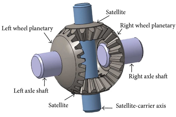
applied to its satellite-carrier axis to rotate it about Figure from G. Antoni, Sci. World J., 2014, 523281
the common axis of two axle shafts, equally to both (2014), adapted with permission. Both satellite gears shafts, even if they rotate with different angular may rotate freely about their common carrier axis.
velocities.
l
2
4.7. The end of a uniform thin rod of length 2 l and mass m, initially at rest, is hit by a bullet of mass m' , flying with a velocity v0 perpendicular to the m
rod (see the figure on the right), which gets stuck in it. Use two different v0
approaches to calculate the velocity of the opposite end of the rod right after
m'
the collision.
4.8. A ball of radius R, initially at rest on a horizontal surface, is hit F t
with a billiard cue in the horizontal direction, at height h above the table –
see the figure on the right. Using the Coulomb approximation for the
0
kinetic friction force between the ball and the surface ( F f = N), calculate h
R
the final linear velocity of the rolling ball as a function of h. Would it matter if the hit point is shifted horizontally (normally to the plane of the
drawing)?
Hint: As in most solid body collision problems, during the short Chapter 4
Page 28 of 32





Essential Graduate Physics
CM: Classical Mechanics
time of the cue hit, all other forces exerted on the ball may be considered negligibly small.
4.9. A round cylinder of radius R and mass M may roll, without slippage, over a horizontal surface. The mass density distribution inside the cylinder is not uniform, so its center of mass is at some distance l 0 from its geometrical axis, and the moment of inertia I (for rotation about the axis parallel to the symmetry axis but passing through the center of mass) is different from MR 2/2, where M is the cylinder’s mass. Derive the equation of motion of the cylinder under the effect of the uniform vertical gravity field, and use it to calculate the frequency of small oscillations of the cylinder near its stable equilibrium position.
4.10. A body may rotate about a fixed horizontal axis – see Fig. 5. Find the frequency of its small oscillations in a uniform gravity field, as a function of the distance l of the axis from the body’s center of mass 0, and analyze the result.
4.11. Calculate the frequency, and sketch the mode of oscillations34
M , R
of a round uniform cylinder of radius R and the mass M, that may roll, without slippage, on a horizontal surface of a block of mass M’. The block, M'
in turn, may move in the same direction, without friction, on an immobile
horizontal surface, being connected to it with an elastic spring – see the figure on the right.
l'
4.12. A thin uniform bar of mass M and length l is hung on a light thread of length
l’ (like a “chime” bell – see the figure on the right). Derive the equations of the system’s M
motion within a vertical plane passing through the suspension point.
l
g
4.13. A uniform round solid cylinder of mass M can roll, R
without slippage, over a concave round cylindrical surface of a block
R'
of mass M’, in a uniform gravity field – see the figure on the right.
M
g
The block can slide without friction on a horizontal surface. Using the
M'
Lagrangian formalism,
(i) find the frequency of small oscillations of the system near the equilibrium, and (ii) sketch the oscillation mode for the particular case M’ = M, R’ = 2 R.
4.14. A uniform solid hemisphere of radius R and mass M is R
placed on a horizontal surface – see the figure on the right. Find the
'
0
frequency of its small oscillations within a vertical plane, for two ultimate
cases:
g
(i) there is no friction between the sphere and the horizontal surface;
(ii) the static friction between them is so strong that there is no slippage.
34 The term mode usually refers to the spatial pattern of oscillations; it will be much discussed in later chapters.
Chapter 4
Page 29 of 32
CM: Classical Mechanics
4.15. For the “sliding ladder” problem started in Sec. 3 (see Fig. 7), find the critical value c of the angle at that the ladder loses its contact with the vertical wall, assuming that it starts sliding from the vertical position, with a negligible initial velocity.
a' ?
4.16. Six similar, uniform rods of length l and mass m are connected by light joints so that they may rotate, without friction, versus each other, forming l, m a planar polygon. Initially, the polygon was at rest, and had the correct hexagon shape – see the figure on the right. Suddenly, an external force F is applied to the middle of one rod, in the direction of the hexagon’s symmetry center.
a ?
Calculate the accelerations: of the rod to which the force is applied ( a), and of the opposite rod ( a’), immediately after the application of the force.
F
ω
4.17. A rectangular cuboid (parallelepiped) with sides a
a
1, a 2, and a 3,
1
a
made of a material with a constant mass density , is rotated with a constant
2
angular velocity about one of its space diagonals – see the figure on the a right. Calculate the torque necessary to sustain this rotation.
3
4.18. A uniform round ball rolls, without slippage, over a “turntable”: a horizontal plane rotated about a vertical axis with a time-independent angular velocity . Derive a self-consistent equation of motion of the ball’s center, and discuss its solutions.
4.19. Calculate the free precession frequency of a uniform thin round disk rotating with an angular velocity about a direction very close to its symmetry axis, from the point of view of: (i) an observer rotating with the disk, and
(ii) a lab-based observer.
4.20. Use the Euler equations to prove the fact mentioned in Sec. 4: free rotation of an arbitrary body (“asymmetric top”) about its principal axes with the smallest and largest moments of inertia is stable, while that about the intermediate- Ij axis is not. Illustrate the same fact using the Poinsot construction.
4.21. Give an interpretation of the torque-induced precession, that would explain its direction, by using a simple system exhibiting this effect, as a model.
4.22. One end of a light shaft of length l is firmly
attached to the center of a thin uniform solid disk of radius R and
R, M
mass M, whose plane is perpendicular to the shaft. Another end
of the shaft is attached to a vertical axis (see the figure on the
l
right) so that the shaft may rotate about the axis without friction.
g
The disk rolls, without slippage, over a horizontal surface so that
the whole system rotates about the vertical axis with a constant angular velocity . Calculate the (vertical) supporting force N exerted on the disk by the surface.
Chapter 4
Page 30 of 32


Essential Graduate Physics
CM: Classical Mechanics
4.23. A coin of radius r is rolled over a horizontal surface, without slippage. Due to its tilt , it rolls around a circle of radius R – see the figure on
the right. Modeling the coin as a very thin round disk, calculate the time period 2 r
of its motion around the circle.
g
0
R
4.24. Solve the previous problem in the limit when the coin tilt angle
and the ratio r/ R are small, by simpler means, using
(i) an inertial ("lab") reference frame, and
(ii) the non-inertial reference frame moving with the coin's center but not rotating with it.
4.25. A symmetric top on a point support (as shown see, e.g., Fig. 9), rotating around its symmetry axis with a high angular velocity rot, is subjected to not only its weight Mg but also an additional force also applied to the top’s center of mass, with its vector rotating in the horizontal plane with a constant angular velocity << rot. Derive the system of equations describing the top’s motion.
Analyze their solution for the simplest case when is exactly equal to the frequency (72) of the torque-induced precession in the gravity field alone.
4.26. Analyze the effect of small friction on a fast rotation of a symmetric top around its axis, using a simple model in that the lower end of the body is a right cylinder of radius R.
4.27. An air-filled balloon is placed inside a water-filled container, which moves by inertia in free space, at negligible gravity. Suddenly, force F is applied to the container, pointing in a certain direction. What direction does the balloon move relative to the container?
4.28. Two planets are in a circular orbit around their common center of mass. Calculate the effective potential energy of a much lighter body (say, a spacecraft) rotating with the same angular velocity, on the line connecting the planets. Sketch the radial dependence of U ef and find out the number of so-called Lagrange points in which the potential energy has local maxima. Calculate their position explicitly in the limit when one of the planets is much more massive than the other one.
4.29. Besides the three Lagrange points L1, L2, and L3 discussed in the previous problem, which are located on the line connecting two planets on circular orbits about their mutual center of mass, there are two off-line points L4 and L5 – both within the plane of the planets’ rotation. Calculate their positions.
4.30. The following simple problem may give additional clarity to the physics of the Coriolis
“force”. A bead of mass m may slide, without friction, along a straight rod that is rotated within a horizontal plane with a constant angular velocity – see the figure on the right. Calculate the bead’s acceleration and the force N exerted on it by the rod, in:
(i) an inertial (“lab”) reference frame, and
(ii) the non-inertial reference frame rotating with the rod (but not moving with the bead), and compare the results.
4.31. Analyze the dynamics of the famous Foucault pendulum used for spectacular demonstrations of the Earth’s rotation. In particular, calculate the angular velocity of the rotation of its Chapter 4
Page 31 of 32


Essential Graduate Physics
CM: Classical Mechanics
oscillation plane relative to the Earth’s surface, at a location with a polar angle (“colatitude”) . Assume that the pendulum oscillation amplitude is small enough to neglect nonlinear effects and that its oscillation period is much shorter than 24 hours.
4.32. A small body is dropped down to the surface of Earth from a height h << R E, without initial velocity. Calculate the magnitude and direction of its deviation from the vertical, due to the Earth’s rotation. Estimate the effect’s magnitude for a body dropped from the Empire State Building.
4.33. Calculate the height of solar tides on a large ocean, using the following simplifying assumptions: the tide period (½ of the Earth's day) is much longer than the period of all ocean waves, the Earth (of mass M E) is a sphere of radius R E, and its distance r S from the Sun (of mass M S) is constant and much larger than R E.
4.34. A satellite is on a circular orbit of radius R, around the Earth. Neglecting the gravity field of the satellite,
(i) write the equations of motion of a small body as observed from the satellite and simplify them for the case when the motion is limited to the satellite’s close vicinity;
(ii) use these equations to prove that a body may be placed on an elliptical trajectory around the satellite’s center of mass, within its plane of rotation around the Earth. Calculate the ellipse’s orientation and eccentricity.
4.35. A non-spherical shape of an artificial satellite may ensure its stable angular orientation relative to the Earth’s surface, advantageous for many practical goals. By modeling a satellite as a strongly elongated, axially-symmetric body moving around the Earth on a circular orbit of radius R, find its stable orientation.
4.36. A rigid, straight, uniform rod of length l, with the lower end on a pivot, falls in a uniform gravity field – see the figure on the right. Neglecting friction, calculate the distribution of the bending torque along its length, and analyze the result.
l
Hint: As will be discussed in detail in Sec. 7.5 of the lecture notes, the bending g
torque’s gradient along the rod’s length is equal to the rod-normal (“shear”) component of the total force between two parts of the rod, mentally separated by its cross-section.
4.37. Let r be the radius vector of a particle, as measured in a possibly non-inertial but certainly non-rotating reference frame. Taking its Cartesian components for the generalized coordinates, calculate the corresponding generalized momentum p of the particle and its Hamiltonian function H. Compare p
with mv, and H with the particle’s energy E. Derive the Lagrangian equation of motion in this approach, and compare it with Eq. (92).
Chapter 4
Page 32 of 32
CM: Classical Mechanics
Chapter 5. Oscillations
In this course, oscillations and waves are discussed in detail, because of their importance for fundamental and applied physics. This chapter starts with a discussion of the harmonic oscillator, whose differential equation of motion is linear and hence allows the full analytical solution, and then proceeds to so-called “nonlinear” and “parametric” systems whose dynamics may be only explored by either approximate analytical or numerical methods.
5.1. Free and forced oscillations
In Sec. 3.2 we briefly discussed oscillations in a keystone Hamiltonian system – a 1D harmonic oscillator described by a very simple Lagrangian1
m
L T ( q) U ( q)
2
2
q q ,
(5.1)
2
2
whose Lagrange equation of motion,2
Harmonic
oscillator:
q
m q
,
0
i.e.
2
q q ,
0
with 2
0 ,
(5.2)
0
0
equation
m
is a linear homogeneous differential equation. Its general solution is given by Eq. (3.16), which is frequently recast into another, amplitude-phase form:
Harmonic
oscillator:
q t
( ) u cos t v sin t A cos
,
(5.3a)
0
0
t
0
motion
where A is the amplitude and is the phase of the oscillations, which are determined by the initial conditions. Mathematically, it is frequently easier to work with sinusoidal functions as complex exponents, by rewriting the last form of Eq. (3a) in one more form:3
i( t )
0
i t 0
q t
( ) Re Ae
Re ae
,
(5.3b)
Real
and where a is the complex amplitude of the oscillations:
complex
amplitudes
a Aei ,
a ,
A
Re a A cos u,
Im a A sin .
v
(5.4)
For an autonomous, Hamiltonian oscillator, Eqs. (3) give the full classical description of its dynamics.
However, it is important to understand that this free-oscillation solution, with a constant amplitude A, 1 For the notation brevity, in this chapter, I will drop indices “ef” in the energy components T and U, and in parameters like m, , etc. However, the reader should still remember that T and U do not necessarily coincide with the actual kinetic and potential energies (even if those energies may be uniquely identified) – see Sec. 3.1.
2 0 is usually called the own frequency of the oscillator. In quantum mechanics, the Germanized version of the same term, eigenfrequency, is used more. In this series, I will use either of the terms, depending on the context.
3 Note that this is the so-called physics convention. Most engineering texts use the opposite sign in the imaginary exponent, exp{- i t} exp{ i t}, with the corresponding sign implications for intermediate formulas but identical final results for real variables.
© K. Likharev
CM: Classical Mechanics
means the conservation of the energy E T + U = A 2/2 of the oscillator. If its energy changes for any reason, the description needs to be generalized.
First of all, if the energy leaks out of the oscillator to its environment (the effect usually called energy dissipation), the free oscillations decay with time. The simplest model of this effect is represented by an additional linear drag (or “kinematic friction”) force, proportional to the generalized velocity and directed opposite to it:
F
q ,
(5.5)
v
where constant is called the drag coefficient.4 The inclusion of this force modifies the equation of motion (2) to become
q
m q q
0 .
(5.6a)
This equation is frequently rewritten in the form
Free
q
oscillator
2 q
2
q ,
0
with
,
(5.6b)
0
2 m
with
damping
where the parameter is called the damping coefficient (or just “damping”). Note that Eq. (6) is still a linear homogeneous second-order differential equation, and its general solution still has the form of the sum (3.13) of two exponents of the type exp{ t}, with arbitrary pre-exponential coefficients. Plugging such an exponent into Eq. (6), we get the following algebraic characteristic equation for : 2
2
2
.
0
(5.7)
0
Solving this quadratic equation, we get
i ' ,
where '
(5.8)
0
0
2 2
0
1/2,
so for not very high damping ( < 0) we get the following generalization of Eq. (3):5
t
q ( t)
c e
c e t u
't v
t
't e
A e t
't (5.9)
free
cos
sin
0
0
0
0
cos
0
0
0 .
The result shows that, besides a certain correction to the free oscillation frequency (which is very small in the most interesting low damping limit, << 0), the energy dissipation leads to an exponential decay of oscillation amplitude with the time constant = 1/:
4 Here Eq. (5) is treated as a phenomenological model, but in statistical mechanics, such dissipative term may be derived as an average force exerted upon a system by its environment, at very general assumptions. As will be discussed in detail later in this series (QM Chapter 7 and SM Chapter 5), due to the numerous degrees of freedom of a typical environment (think about the molecules of air surrounding a macroscopic pendulum), its force also has a random component; as a result, the dissipation is fundamentally related to fluctuations. The latter effect may be neglected (as it is in this course) only if the oscillator’s energy E is much higher than the energy scale of its random fluctuations – in the thermal equilibrium at temperature T, the larger of k B T and 0/2.
5 Systems with high damping ( > 0) can hardly be called oscillators, and though they are used in engineering and physical experiment (e.g., for shock and sound isolation), due to the lack of time/space, for their detailed discussion I have to refer the interested reader to special literature – see, e.g., C. Harris and A. Piersol, Shock and Vibration Handbook, 5th ed., McGraw Hill, 2002. Let me only note that according to Eq. (8), the dynamics of systems with very high damping ( >> 0) has two very different time scales: a relatively short “momentum relaxation time” 1/
2
- 1/2 = m/, and a much longer “coordinate relaxation time” 1/+. 2/0 = /-.
Chapter 5
Page 2 of 38
CM: Classical Mechanics
Decaying
t
/
1
2 m
free
A A e
,
where
.
(5.10)
0
oscillations
A very popular dimensionless measure of damping is the so-called quality factor Q (or just the Q- factor) which is defined as 0/2, and may be rewritten in several other useful forms:
m
m
0
0
1/2
0
Q
,
(5.11)
2
T
2
where T 2 π/0 is the oscillation period in the absence of damping – see Eq. (3.29). Since the oscillation energy E is proportional to A 2, i.e. decays as exp{-2 t/}, i.e. with the time constant /2, the last form of Eq. (11) may be used to rewrite the Q-factor in one more form: E
E
Q
,
(5.12)
0 E
0 P
where P is the energy dissipation rate. (Other practical ways to measure Q will be discussed below.) The range of Q-factors of mechanical oscillators is very broad, from Q ~ 10 for a human leg (with relaxed muscles), to Q ~ 104 of the quartz crystals used in electronic clocks and watches, and all the way up to Q > 1010 for nanoparticles suspended (by electrostatic forces) in high vacuum.
In contrast to the decaying free oscillations, forced oscillations induced by an external force F( t), may maintain their amplitude (and hence energy) infinitely, even at non-zero damping. This process may be described using a still linear but now inhomogeneous differential equation q
m q q
F( t),
(5.13a)
or, more usually, the following generalization of Eq. (6b):
Forced
oscillator
with
q 2 q
2
q f t(),
where f t
( ) F t
( ) / m .
(5.13b)
0
damping
For a mechanical linear, dissipative 1D oscillator (6), under the effect of an additional external force F( t), Eq. (13a) is just an expression of the 2nd Newton law. However, according to Eq. (1.41), Eq. (13) is valid for any dissipative, linear 6 1D system whose Gibbs potential energy (1.39) has the form U G( q, t) =
κq 2/2 – F( t) q.
The forced-oscillation solutions to Eq. (13) may be analyzed by two mathematically equivalent methods whose relative convenience depends on the character of function f( t).
(i) Frequency domain. Representing the function f( t) as a Fourier sum of sinusoidal harmonics:7
f ( t)
i t
f e
,
(5.14)
and using the linearity of Eq. (13), we may represent its general solution as a sum of the decaying free oscillations (9) with the frequency 0 ’, that are independent of the function f( t), and forced oscillations due to each of the Fourier components of the force:8
6 This is a very unfortunate, but common jargon, meaning “the system described by linear equations of motion”.
7 Here, in contrast to Eq. (3b), we may drop the operator Re, assuming that f- = f*, so that the imaginary components of the sum compensate for each other.
Chapter 5
Page 3 of 38
CM: Classical Mechanics
General
i t
q t
( ) q
t
( ) q
t
( ), q
t
( )
.
(5.15) solution
free
forced
forced
a e
of Eq. (13)
Plugging Eq. (15) into Eq. (13), and requiring the factors before each e-i t on both sides to be equal, we get
a
(),
f
(5.16)
where the complex function (), in our particular case equal to
1
()
(5.17)
2
2
i
0
,
2
is called either the response function or (especially for non-mechanical oscillators) the generalized susceptibility. From here, and Eq. (4), the amplitude of the oscillations under the effect of a sinusoidal force is
1
A a f () ,
with ()
Forced
.
(5.18)
2
2 2
2
( ) (2 )
oscillations
0
1/2
This formula describes, in particular, an increase of the oscillation amplitude A at 0 – see the left panel of Fig. 1. In particular, at the exact equality of these two frequencies, 1
( )
,
(5.19)
0
2
0
so, according to Eq. (11), the ratio of the response magnitudes at =
2
0 and = 0 (()=0 = 1/0 ) is
exactly equal to the Q-factor of the oscillator. Thus, the response increase is especially strong in the low-damping limit ( << 0, i.e. Q >> 1); moreover, at Q and 0, the response diverges. (This mathematical fact is very useful for the methods to be discussed later in this section.) This is the classical description of the famous phenomenon of resonance, so ubiquitous in physics.
15
1
Q
Q 100
100
10
0.75
10
5
()
10
2
0.5
(0)
1
0.25
5
5
2
0
1
0
0.5
1
1.5
2
/ 0
0
Fig. 5.1. Resonance in the linear
0
0.5
1
1.5
2
oscillator, for several values of Q.
/ 0
8 In physics, this mathematical property of linear equations is frequently called the linear superposition principle.
Chapter 5
Page 4 of 38
CM: Classical Mechanics
Due to the increase of the resonance peak height, its width is inversely proportional to Q.
Quantitatively, in the most interesting low-damping limit, i.e. at Q >> 1, the reciprocal Q-factor gives the normalized value of the so-called full-width at half-maximum (FWHM) of the resonance curve:9
1
.
(5.20)
Q
0
Indeed, this is defined as the difference (+ – –) between such two values of at that the modulus squared of the oscillator response function, ()2 (which is proportional to the oscillation energy), equals a half of its resonance value (19). In the low damping limit, these points are very close to 0, so in the linear approximation in –
2
0 << 0, we may write (0 – 2) –( +0)( – 0) –2 –
20, where
(5.21)
0
is a convenient parameter called detuning, which will be repeatedly used later in this chapter, and beyond it. In this approximation, the second of Eqs. (18) is reduced to10
1
2
()
.
(5.22)
2
4
0 2
2
As a result, the points correspond to 2 = δ 2, i.e. ω = ω 0 ± δ = ω 0(1 ± 1/2 Q), so ω+ – ω- =
ω 0/ Q, thus proving Eq. (20).
(ii) Time domain. Returning to an arbitrary external force f( t), one may argue that Eqs. (9), (15)-
(17) provide a full solution of the forced oscillation problem even in this general case. This is formally correct, but this solution may be very inconvenient if the external force is far from a sinusoidal function of time, especially if it is not periodic at all. In this case, we should first calculate the complex amplitudes f participating in the Fourier sum (14). In the general case of a non-periodic f( t), this is actually the Fourier integral,11
f t
( )
f e i t dt
,
(5.23)
so f should be calculated using the reciprocal Fourier transform,
1
f
f t' () ei t'dt' .
(5.24)
2
Now we may use Eq. (16) for each Fourier component of the resulting forced oscillations, and rewrite the last of Eqs. (15) as
9 Note that the phase shift arg[()] between the oscillations and the external force (see the right panel in Fig.
1) makes its steepest change, by /2, within the same frequency interval .
10 Such function of frequency may be met in many branches of science, frequently under special names, including the “Cauchy distribution”, “the Lorentz function” (or “Lorentzian line”, or “Lorentzian distribution”), “the Breit-Wigner function” (or “the Breit-Wigner distribution”), etc.
11 Let me hope that the reader knows that Eq. (23) may be used for periodic functions as well; in such a case, f is a set of equidistant delta functions. (A reminder of the basic properties of the Dirac δ-function may be found, for example, in MA Sec. 14.)
Chapter 5
Page 5 of 38
CM: Classical Mechanics
i t
i t
1
q
( t) a e
d () f e
d d ()
dt' f ( t' ) i( t' t)
e
forced
2
(5.25)
1
dt' f ( t' )
i t'
d ()
(
t)
e
,
2
with the response function ( ω) given, in our case, by Eq. (17). Besides requiring two integrations, Eq.
(25) is conceptually uncomforting: it seems to indicate that the oscillator’s coordinate at time t depends not only on the external force exerted at earlier times t’ < t, but also at future times. This would contradict one of the most fundamental principles of physics (and indeed, science as a whole), causality: no effect may precede its cause.
Fortunately, a straightforward calculation (left for the reader’s exercise) shows that the response function (17) satisfies the following rule:12
()
e i
d
,
0
for
0.
(5.26)
This fact allows the last form of Eq. (25) to be rewritten in either of the following equivalent forms: t
Linear
q
t
( )
f t'
( ) G t
( t' ) dt' f t
( ) G
( ) d ,
(5.27) system’s
forced
response
0
where G( τ), defined as the Fourier transform of the response function,
1
Temporal
G
i
( e ω
)
d ,
(5.28) Green’s
2
function
is called the ( temporal) Green’s function of the system. According to Eq. (26), G( τ) = 0 for all τ < 0.
While the second form of Eq. (27) is frequently more convenient for calculations, its first form is more suitable for physical interpretation of the Green’s function. Indeed, let us consider the particular case when the force is a delta function
f ( t) ( t t' ),
with t' t
i.e.
,
t t' 0 ,
(5.29)
representing an ultimately short pulse at the moment t’, with unit “area” f( t) dt. Substituting Eq. (29a) into Eq. (27),13 we get
q t G t t' .
(5.30)
Thus Green’s function G( t – t’) is just the oscillator’s response, as measured at time t, to a short force pulse of unit “area”, exerted at time t’. Hence Eq. (27) expresses the linear superposition principle in the time domain: the full effect of the force f( t) on a linear system is a sum of the effects of short pulses of duration dt’ and magnitude f( t’), each with its own “weight” G( t – t’) – see Fig. 2.
12 Eq. (26) is true for any linear physical system in which f( t) represents a cause, and q( t) its effect. Following tradition, I discuss the frequency-domain expression of this causality relation (called the Kramers-Kronig relations) in the Classical Electrodynamics part of this lecture series – see EM Sec. 7.2.
13 Technically, for this integration, t’ in Eq. (27) should be temporarily replaced with another letter, say t” .
Chapter 5
Page 6 of 38
CM: Classical Mechanics
G t t'
f ( t' )
Fig. 5.2. A schematic, finite-interval
q( t)
representation of a force f( t) as a sum of
. . .
. . .
short pulses at all times t’ < t, and their
contributions to the linear system’s
response q( t), as given by Eq. (27).
t
t'
0
dt'
This picture may be used for the calculation of Green’s function for our particular system.
Indeed, Eqs. (29)-(30) mean that G() is just the solution of the differential equation of motion of the system, in our case, Eq. (13), with the replacement t , and a δ-functional right-hand side: 2
d G( )
dG( )
2
2
G( ) ( ) .
(5.31)
2
0
d
d
Since Eqs. (27) describes only the second term in Eq. (15), i.e. only the forced, rather than free oscillations, we have to exclude the latter by solving Eq. (31) with zero initial conditions: dG
G 0
0 ,0
(5.32)
d
where = – 0 means the instant immediately preceding = 0.
This problem may be simplified even further. Let us integrate both sides of Eq. (31) over an infinitesimal interval including the origin, e.g. [– d /2, + d /2], and then follow the limit d 0. Since Green’s function has to be continuous because of its physical sense as the (generalized) coordinate, all terms on the left-hand side but the first one vanish, while the first term yields dG/d+0 – dG/ d–0. Due to the second of Eqs. (32), the last of these two derivatives has to equal zero, while the right-hand side of Eq. (31) yields 1 upon the integration. Thus, the function G() may be calculated for > 0 (i.e. for all times when it is different from zero) by solving the homogeneous version of the system’s equation of motion for > 0, with the following special initial conditions:
dG
G0 ,
0
0 .1
(5.33)
d
This approach gives us a convenient way for the calculation of Green’s functions of linear systems. In particular for the oscillator with not very high damping ( < 0, i.e. Q > ½), imposing the boundary conditions (33) on the homogeneous equation’s solution (9), we immediately get Oscillator’s
1
Green’s
G
( )
e
sin ' .
(5.34)
function
'
0
0
(The same result may be obtained directly from Eq. (28) with the response function () given by Eq.
(19). This way is, however, a little bit more cumbersome, and is left for the reader’s exercise.) Relations (27) and (34) provide a very convenient recipe for solving many forced oscillations problems. As a very simple example, let us calculate the transient process in an oscillator under the effect of a constant force being turned on at t = 0, i.e. proportional to the Heaviside step function: Chapter 5
Page 7 of 38
CM: Classical Mechanics
,
0
for t ,
0
f ( t) f t
(5.35)
0
f , for t ,
0
0
provided that at t < 0 the oscillator was at rest, so in Eq. (15), q free( t) 0. Then the second form of Eq.
(27), together with Eq. (34), yield
t
1
q( t) f ( t ) G( ) d
f
e
sin ' d.
(5.36)
0
0
'
0
0
0
The simplest way to work out such integrals is to represent the sine function under it as the imaginary part of exp{ i0 ’t}, and merge the two exponents, getting
1
t
1
i '
F
0
0
t
q t
( ) f
Im
e
1
cos
sin
. (5.37)
0
e
't
't
0
0
'
0
i ' 0
k
0
' 0
This result, plotted in Fig. 3, is rather natural: it describes nothing more than the transient from the initial position q = 0 to the new equilibrium position q
2
0 = f 0/0 = F 0/, accompanied by decaying
oscillations. For this particular simple function f( t), the same result might be also obtained by introducing a new variable q~ t q( t) – q 0 and solving the resulting homogeneous equation for q~ (with appropriate initial condition q~ (0) = – q 0). However, for more complicated functions f( t), Green’s function approach is irreplaceable.
2
1.5
q( t)
1
q 0
0.5
Fig. 5.3. The transient process in a linear
oscillator, induced by a step-like force f( t), for
the particular case /
0
0 = 0.1 (i.e., Q = 5).
0
20
40
t
0
Note that for any particular linear system, its Green’s function should be calculated only once, and then may be repeatedly used in Eq. (27) to calculate the system response to various external forces –
either analytically or numerically. This property makes Green’s function approach very popular in many other fields of physics – with the corresponding generalization or re-definition of the function.14
5.2. Weakly nonlinear oscillations
In comparison with systems discussed in the last section, which are described by linear differential equations with constant coefficients and thus allow a complete and exact analytical solution, oscillations in nonlinear systems (very unfortunately but commonly called nonlinear oscillations) present a complex and, generally, analytically intractable problem. However, much insight into possible 14 See, e.g., Sec. 6.6, and also EM Sec. 2.7 and QM Sec. 2.2.
Chapter 5
Page 8 of 38
CM: Classical Mechanics
processes in such systems may be gained from a discussion of an important case of weakly nonlinear systems, which may be explored analytically. An important example of such systems is given by an anharmonic oscillator – a 1D system whose higher terms in the potential’s expansion (3.10) cannot be neglected, but are small and may be accounted for approximately. If, in addition, damping is low (or negligible), and the external harmonic force exerted on the system is not too large, the equation of motion is a slightly modified version of Eq. (13):
Weakly
nonlinear
2
q q f ( t, q, q,...) ,
(5.38)
oscillator
where 0 is the anticipated frequency of oscillations (whose choice may be to a certain extent arbitrary – see below), and the right-hand side f is small (say, scales as some small dimensionless parameter << 1), and may be considered as a small perturbation.
Since at = 0, this equation has the sinusoidal solution given by Eq. (3), one might naïvely think that at a nonzero but small , the approximate solution to Eq. (38) should be sought in the form Perturbative
solution
(0)
)
1
(
(2)
( n)
n
q t
( ) q q q ...,
q
where
,
(5.39)
with q(0) = A cos(0 t – ) 0. This is a good example of apparently impeccable mathematical reasoning that would lead to a very inefficient procedure. Indeed, let us apply it to the problem we already know the exact solution for, namely free oscillations in a linear but damped oscillator, for this occasion assuming the damping to be very low, /0 ~ << 1. The corresponding equation of motion, Eq. (6), may be represented in form (38) if we take = 0 and
f
2 q,
with .
(5.40)
The naïve perturbation theory based on Eq. (39) would allow us to find small corrections, of the order of
, to the free, non-decaying oscillations A cos(0 t – ). However, we already know from Eq. (9) that the main effect of damping is a gradual decrease of the free oscillation amplitude to zero, i.e. a very large change of the amplitude, though at low damping, << 0, this decay takes large time t ~ >> 1/0.
Hence, if we want our approximate method to be productive (i.e. to work at all time scales, in particular for forced oscillations with stationary amplitude and phase), we need to account for the fact that even a small right-hand side of Eq. (38) may eventually lead to large changes of oscillation’s amplitude A (and sometimes, as we will see below, also of oscillation’s phase ) at large times, because of the slowly accumulating effects of the small perturbation.15
This goal may be achieved16 by the account of these slow changes already in the “0th approximation”, i.e. the basic part of the solution in the expansion (39):
15 The same flexible approach is necessary for approximations used in quantum mechanics. The method discussed here is closer in spirit (though not completely identical) to the WKB approximation (see, e.g., QM Sec.
2.4) rather than most perturbative approaches (QM Ch. 6).
16 This approach has a long history and, unfortunately, does not have a commonly accepted name. It had been gradually developed in celestial mechanics, but its application to 1D systems (on which I am focusing) was clearly spelled out only in 1926 by Balthasar van der Pol. So, I will follow several authors who call it the van der Pol method. Note, however, that in optics and quantum mechanics, this method is commonly called the Rotating Wave Approximation (RWA). In math-oriented texts, this approach, and especially its extensions to higher approximations, is usually called either the small parameter method or the asymptotic method. The list of other Chapter 5
Page 9 of 38
CM: Classical Mechanics
(0)
q
(
A t) cos[ t ( t)],
with ,
A at
0
0 .
(5.41) 0th
approximation
(It is evident that Eq. (9) is a particular case of this form.) Let me discuss this approach using a simple but representative example of a dissipative (but high- Q) pendulum driven by a weak sinusoidal external force with a nearly resonant frequency:
q 2
2
q
sin q f cos t
,
(5.42)
0
0
with | ω – ω 0|, δ << ω 0, and the force amplitude f 0 so small that | q | << 1 at all times. From what we know about the forced oscillations from Sec. 1, in this case, it is natural to identify on the left-hand side of Eq. (38) with the force’s frequency. Expanding sin q into the Taylor series in small q, keeping only the first two terms of this expansion, and moving all small terms to the right-hand side, we can rewrite Eq. (42) in the following popular form (38):17
2
q q 2 q
2
3
q
q f cos t f ( t, q, q) .
(5.43) Duffing
0
equation
Here = 2
0 /6 in the case of the pendulum (though the calculations below will be valid for any α), and the second term on the right-hand side was obtained using the approximation already employed in Sec.
1: (2 – 2
0 ) q 2 ( – 0) q = 2 q, where – 0 is the detuning parameter that was already used earlier – see Eq. (21).
Now, following the general recipe expressed by Eqs. (39) and (41), in the 1st approximation in f
we may look for the solution to Eq. (43) in the following form:
q( t) A cos Ψ
)
1
(
q ( t),
Ψ
where
t ,
)
1
(
q
~ .
(5.44)
Let us plug this solution into both parts of Eq. (43), keeping only the terms of the first order in . Thanks to our (smart :-) choice of on the left-hand side of that equation, the two zero-order terms in that part cancel each other. Moreover, since each term on the right-hand side of Eq. (43) is already of the order of
, we may drop q(1) from the substitution into that part at all, because this would give us only terms O(2) or higher. As a result, we get the following approximate equation: d
)
1
(
2
)
1
(
(0)
q q f t 2
( A cos ) 2 A cos A cos 3 f cos t. (5.45) 0
dt
According to Eq. (41), generally, A and should be considered (slow) functions of time.
However, let us leave the analyses of the transient process and system’s stability until the next section, and use Eq. (45) to find stationary oscillations in the system, that are established after an initial transient process. For that limited task, we may take A = const, = const, so q(0) represents sinusoidal oscillations of frequency . Sorting the terms on the right-hand side according to their time dependence,18 we see that it has terms with frequencies and 3:
scientists credited for the development of this method, its variations, and extensions includes, most notably, N.
Krylov, N. Bogolyubov, and Yu. Mitroplolsky.
17 This equation is frequently called the Duffing equation (or the equation of the Duffing oscillator), after Georg Duffing who carried out its first (rather incomplete) analysis in 1918.
18 Using the second of Eqs. (44), cos t may be rewritten as cos ( + ) cos cos – sin sin . Then using the identity given, for example, by MA Eq. (3.4): cos3 = (3/4)cos + (1/4)cos 3, we get Eq. (46).
Chapter 5
Page 10 of 38
CM: Classical Mechanics
(0)
3
3
1
f
2 A
A f cos cosΨ
A
f
A
(5.46)
0
2
sin
0
sin Ψ
3 cos
.
Ψ
3
4
4
Now comes the main punch of the van der Pol approach: mathematically, Eq. (45) may be viewed as the equation of oscillations in a linear, dissipation-free harmonic oscillator of own frequency
(not 0!) under the action of an external force f (0)( t). In our particular case, this force is given by Eq.
(46) and has three terms: two “quadrature” components with that very frequency , and the third one with frequency 3. As we know from our analysis of this problem in Sec. 1, if any of the first two components is not equal to zero, q(1) grows to infinity – see Eq. (19) with = 0. At the same time, by the very structure of the van der Pol approximation, q(1) has to be finite – moreover, small! The only way to avoid these infinitely growing (so-called secular) terms is to require that the amplitudes of both quadrature components of f (0) with frequency are equal to zero:
3
2
3
A A f cos ,
0
2 A f sin .
0
(5.47)