

Classical Electrodynamics by Konstantin K. Likharev - HTML preview
Download the book in PDF, ePub, Kindle for a complete version.
A
rd
C
r
dA
Fig. 5.11. Calculating the
magnetic dipole moment
0
of a planar current loop.
I
The comparison of Eqs. (96) and (97) allows a useful estimate of atomic currents, by finding what current I should flow in a circular loop of the atomic size scale (the Bohr radius) r B ~ 0.510-10 m, i.e. of area A ~ 10-20 m2, to produce a magnetic moment of the order of B.42 The result is surprisingly macroscopic: I ~ 1 mA – quite comparable to the current driving the sound in your phone’s earbuds.
Though due to the quantum-mechanical spread of electron wavefunctions, this estimate should not be taken too literally, it is very useful for getting a gut feeling of how significant the atomic magnetism is, and hence why ferromagnets may provide such strong magnetic fields.
After these illustrations, let us return to the discussion of the general Eq. (90). Plugging it into (also general) Eq. (27), we may calculate the magnetic field of a magnetic dipole: 43
42 Another way to arrive at the same estimate is to take I ~ ef = e/2 with ~ 1016 s-1 being the typical frequency of radiation due to atomic interlevel quantum transitions.
43 Similarly to the situation with the electric dipoles (see Eq. (3.24) and its discussion), it may be shown that the magnetic field of any closed current loop (or any system of such loops) satisfies the following equality: B r 3
( ) d r 2 /
3 m
,
0
V
where the integral is over any sphere confining all the currents. On the other hand, as we know from Sec. 3.1, for a field with the structure (99), derived from the long-range approximation (90), such an integral vanishes. As a result, to get a coarse-grain description of the magnetic field of a small system located at r = 0, that would give the correct average value of the magnetic field, Eq. (99) should be modified as follows:
r
3 r
( m)
2
r
0
8
B
r
( )
m
m
,
cg
r
5
4
r
3
in a conceptual (though not quantitative) similarity to Eq. (3.25).
Chapter 5
Page 23 of 42
EM: Classical Electrodynamics
2
3r(r m) m r
Magnetic
0
B(r)
.
(5.99) dipole’s
5
4
r
field
The structure of this formula exactly replicates that of Eq. (3.13) for the electric dipole field – including the sign). Because of this similarity, the energy of a dipole of a fixed magnitude m in an external field, and hence the torque and the force exerted on it by a fixed external field, are given by expressions fully similar to those for an electric dipole – see Eqs. (3.15)-(3.19):44
Magnetic
U m
B ,
(5.100) dipole
ext
in external
and as a result,
field
τ m B ,
(5.101)
ext
F (m B ) .
(5.102)
ext
Now let us consider a system of many magnetic dipoles (e.g., atoms or molecules), distributed in space with an atomic-scale-averaged density n. Then we can use Eq. (90) generalized in an evident way for an arbitrary position r ’ of the dipole, and the linear superposition principle, to calculate the macroscopic vector potential A:
M(r ) (r r )
0
'
'
A(r)
d 3 r' ,
(5.103)
4
r ' 3
r
where M nm is the magnetization: the average magnetic moment per unit volume. Transforming this integral absolutely similarly to how Eq. (3.27) had been transformed into Eq. (3.29), we get:
' M '
r
0
( )
A(r)
3
d r' .
(5.104)
4
r '
r
Comparing this result with Eq. (28), we see that M is equivalent, in its magnetic effect, to the density jef of a certain effective “magnetization current”. Just as the electric-polarization charge ef discussed in Sec. 3.2 (see Fig. 3.4), the vector jef = M may be interpreted as the uncompensated part of the loop currents representing single magnetic dipoles m – see Fig. 12. Note, however, that since the atomic magnetic dipoles may be due to particles’ spins, rather than the actual electric currents due to the orbital motion, the magnetization current’s nature is not as direct as that of the polarization charge.
j
ef
Fig. 5.12. A cartoon illustrating the physical nature of
the effective magnetization current j
ef = M.
44 Note that the fixation of m and Bext effectively means that the currents producing them are fixed – please have one more look at Eqs. (35) and (97). As a result, Eq. (100) is a particular case of Eq. (53) rather than (54) – hence the minus sign.
Chapter 5
Page 24 of 42
EM: Classical Electrodynamics
Now, using Eq. (28) to add the possible contribution from the stand-alone currents j not included in the currents of microscopic magnetic dipoles, we get the general expression for the vector potential of the macroscopic field:
(
j r )
M(r )
0
' '
'
A(r)
d 3 r' .
(5.105)
4
r '
r
Repeating the calculations that have led us from Eq. (28) to the Maxwell equation (35), with the account of the magnetization current term, for the macroscopic magnetic field B we get
B
.
(5.106)
0 j M
Following the same reasoning as in Sec. 3.2, we may recast this equation as
H j,
(5.107)
where the field defined as
B
Magnetic
H
M ,
(5.108)
field H
0
for historic reasons (and very unfortunately) is also called the magnetic field.45 This is why it is crucial to remember that the physical sense of field H is very much different from field B. To understand this difference better, let us use Eq. (107) to bring Eqs. (3.32), (3.36), (29), and (107) together, writing them as the following system of macroscopic Maxwell equations (again, so far for the stationary case / t =
0):46
Stationary
E ,
0
H , j
macroscopic
(5.109)
Maxwell
D ,
B 0.
equations
These equations clearly show that the roles of the vector fields D and H are very similar: they both may be called “would-be fields” – meaning the fields that would be induced by the stand-alone charges and currents j, if the medium had not modified them by its dielectric and magnetic polarization.
Despite this similarity, let me note an important difference of signs in the relation (3.33) between E, D, and P, on one hand, and the relation (108) between B, H, and M, on the other hand. This is not just a matter of definition. Indeed, due to the similarity of Eqs. (3.15) and (100), including similar signs, the electric and magnetic fields both try to orient the corresponding dipole moments along the field.
Hence, in the media that allow such an orientation (and as we will see momentarily, for magnetic media it is not always the case), the induced polarizations P and M are directed along, respectively, the vectors E and B of the genuine (though macroscopic, i.e. atomic-scale-averaged) fields. According to Eq. (3.33), if the would-be field D is fixed – say, by a fixed stand-alone charge distribution (r) – such a polarization reduces the electric field E = (D – P)/0. On the other hand, Eq. (108) shows that in a magnetic media with a fixed would-be field H, the magnetic polarization making M parallel to B, 45 This confusion is exacerbated by the fact that in Gaussian units, Eq. (108) has the form H = B – 4M, and hence the fields B and H have the same dimensionality (and are formally equal in free space!) – though the unit of H has a different name ( oersted, abbreviated as Oe). Mercifully, in the SI units, the dimensionality of B and H is different, with the unit of H called the ampere per meter.
46 Let me remind the reader once again that in contrast with the system (36) of the Maxwell equations for the genuine (microscopic) fields, the right-hand sides of Eqs. (109) represent only the stand-alone charges and currents, not included in the microscopic electric and magnetic dipoles.
Chapter 5
Page 25 of 42
EM: Classical Electrodynamics
enhances the magnetic field B = 0(H + M). This difference may be traced back to the sign difference in the basic relations (1) and (2), i.e. to the fundamental fact that the electric charges of the same sign repulse, while the currents of the same direction attract each other.
5.5. Magnetic materials
In order to form a complete system, sufficient for the calculation of all fields from given (r) and j(r), the macroscopic Maxwell equations (109) have to be complemented with the constitutive relations describing the medium: D E, j E, and B H. The first two of them were discussed, in brief, in the last two chapters; let us proceed to the last one.
A major difference between the dielectric and magnetic constitutive relations D(E) and B(H) is that while a dielectric medium always reduces the external field, magnetic media may either reduce or enhance it. To quantify this fact, let us consider the most common case – linear magnetic materials in that M (and hence H) is proportional to B. For isotropic materials, this proportionality is characterized by a scalar – either the magnetic permeability defined by the following relation: B H
,
(5.110) Magnetic
permeability
or the magnetic susceptibility 47 defined as
M H .
(5.111) Magnetic
m
susceptibility
Plugging these relations into Eq. (108), we see that these two parameters are not independent, but are related as
1
( ) .
(5.112)
m
0
m vs.
Note that despite the superficial similarity between Eqs. (110)-(112) and the corresponding relations (3.43)-(3.47) for linear dielectrics:
D ,
E
P
,
E
1 ,
(5.113)
e 0
e 0
there is an important conceptual difference between them. Namely, while the vector E on the right-hand sides of Eqs. (113) is the actual (though macroscopic) electric field, the vector H on the right-hand side of Eqs. (110)-(111) represents a “would-be” magnetic field, in most aspects similar to D rather than E –
see, for example, Eqs. (109). This historic difference in the traditional form of the constitutive relations for the electric and magnetic fields is not without its physical reasons. Most experiments with electric and magnetic materials are performed by placing their samples into nearly uniform electric and magnetic fields, and the simplest systems for their implementation are, respectively, plane capacitors (Fig. 2.3) and long solenoids (Fig. 6). The field in the former system may be most conveniently 47 According to Eqs. (110) and (112), i.e. in the SI units, m is dimensionless, while has the same dimensionality as 0. In the Gaussian units, is dimensionless: ()Gaussian = ()SI/0, and m is also introduced differently, as = 1
+ 4m, Hence, just as for the electric susceptibilities, these dimensionless coefficients are different in the two systems: (m )SI = 4(m)Gaussian. Note also that m is formally called the volumic magnetic susceptibility, to distinguish it from the atomic (or “molecular”) susceptibility defined by a similar relation, m H, where m is the induced magnetic moment of a single dipole – e.g., an atom. ( is an analog of the electric atomic polarizability – see Eq. (3.48) and its discussion.) In a dilute medium, i.e. in the absence of substantial dipole-dipole interactions, m = n, where n is the dipole density.
Chapter 5
Page 26 of 42
EM: Classical Electrodynamics
controlled by fixing the voltage V between its plates, which is proportional to the electric field E. On the other hand, the field provided by the solenoid may be fixed by the current I in it, and according to Eq.
(107), the field proportional to this stand-alone current is H, rather than B.48
Table 1 lists the approximate magnetic susceptibility values for several materials. It shows that in contrast to linear dielectrics whose susceptibility e is always positive, i.e. the dielectric constant =
e + 1 is always larger than 1 (see Table 3.1), linear magnetic materials may be either paramagnets (with m > 0, i. e. > 0) or diamagnets (with m < 0, i.e. < 0).
Table 5.1. Susceptibility (
m)SI of a few representative and/or important magnetic materials(a)
“Mu-me
tal” (75% Ni + 15% Fe + a few %% of Cu and Mo)
~20,000(b)
Perm
alloy (80% Ni + 20% Fe)
~8,000(b)
“Electrical” (or “transform
er”) steel (Fe + a few %% of Si)
~4,000(b)
Nickel
~100
Aluminum
+210-5
Oxygen (at am
bient conditions)
+0.210-5
Water
–0.910-5
Diamond
–210-5
Copper
–710-5
Bism
uth (the strongest non-superconducting diamagnet)
–1710-5
(a)
The table does not include bulk superconductors, which may be described, in a so-called coarse-scale approximation, as perfect diamagnets (with B = 0, i.e. formally with m = –1 and = 0), though the actual physics of this phenomenon is different – see Sec. 6.3 below.
(b)
The exact values of m >> 1 for soft ferromagnetic materials (see, e.g., the upper three rows of the table) depend not only on their composition but also on their thermal processing (“annealing”).
Moreover, due to unintentional vibrations, the extremely high values of
m of such materials may
decay with time, though they may be restored to the original values by new annealing. The reason for such behavior is discussed in the text below.
The reason for this difference is that in dielectrics, two different polarization mechanisms (schematically illustrated by Fig. 3.7) lead to the same sign of the average polarization – see the discussion in Sec. 3.3. One of these mechanisms, illustrated by Fig. 3.7b, i.e. the ordering of spontaneous dipoles by the applied field, is also possible for magnetization – for the atoms and molecules with spontaneous internal magnetic dipoles of magnitude m 0 ~ B, due to their net spins.
Again, in the absence of an external magnetic field the spins, and hence the dipole moments m0 may be disordered, but according to Eq. (100), the external magnetic field tends to align the dipoles along its direction. As a result, the average direction of the spontaneous elementary moments m0, and hence the direction of the arising magnetization M, is the same as that of the microscopic field B at the points of the dipole location (i.e., for a diluted media, of H B/0), resulting in a positive susceptibility m, i.e. in the paramagnetism, such as that of oxygen and aluminum – see Table 1.
48 This fact also explains the misleading term “magnetic field” for H.
Chapter 5
Page 27 of 42

Essential Graduate Physics
EM: Classical Electrodynamics
However, in contrast to the electric polarization of atoms/molecules with no spontaneous electric dipoles, which gives the same sign of e – 1 (see Fig. 3.7a and its discussion), the magnetic materials with no spontaneous atomic magnetic dipole moments have m < 0 – the effect called the orbital (or
“Larmor”49) diamagnetism. As the simplest model of this effect, let us consider the orbital motion of an atomic electron about an atomic nucleus as that of a classical particle of mass m 0, with an electric charge q, about an immobile attracting center. As classical mechanics tells us, the central attractive force does not change the particle’s angular momentum L m 0rv, but the applied magnetic field B (that may be taken uniform on the atomic scale) does, due to the torque (101) it exerts on the magnetic moment (95): L
d
q
τ m B
L B .
(5.114)
dt
2 m 0
The diagram in Fig. 13 shows that in the limit of a relatively weak field, when the magnitude of the angular momentum L may be considered constant, this equation describes the rotation (called the torque-induced precession 50) of the vector L about the direction of the vector B, with the angular frequency = – qB/2 m 0, independent of the angle . According to Eqs. (91) and (114), the resulting additional (field-induced) magnetic moment m q – q 2B/ m 0 has, irrespectively of the sign of q, a direction opposite to the field. Hence, according to Eq. (111) with H B/0, the susceptibility m
m/H is indeed negative. (Let me leave its quantitative estimate within this classical model for the reader’s exercise.) The quantum-mechanical treatment confirms this qualitative picture of the Larmor diamagnetism, giving only quantitative corrections to the classical result for m.51
B
L sin
L
dL / dt
v
0
m , q
0
Fig. 5.13. The torque-induced precession of a
m
classical charged particle in a magnetic field.
A simple estimate (also left for the reader’s exercise) shows that in atoms with spontaneous nonzero net spins, the magnetic dipole orientation mechanism prevails over the orbital diamagnetism, so the materials incorporating such atoms usually exhibit net paramagnetism – see Table 1. Due to possible strong quantum interaction between the spin dipole moments, the magnetism of such materials is rather complex, with numerous interesting phenomena and elaborate theories. Unfortunately, all this physics is well outside the framework of this course, and I have to refer the interested reader to special literature,52
but still will mention some key facts.
49 Named after Sir Joseph Larmor who was the first (in 1897) to describe this effect mathematically.
50 For a detailed discussion of this effect see, e.g., CM Sec. 4.5.
51 See, e.g., QM Sec. 6.4. Quantum mechanics also explains why in most common ( s-) ground states, the average contribution (95) of the orbital angular momentum L to the net vector m vanishes.
52 See, e.g., D. J. Jiles, Introduction to Magnetism and Magnetic Materials, 2nd ed., CRC Press, 1998, or R. C.
O’Handley, Modern Magnetic Materials, Wiley, 1999.
Chapter 5
Page 28 of 42
Essential Graduate Physics
EM: Classical Electrodynamics
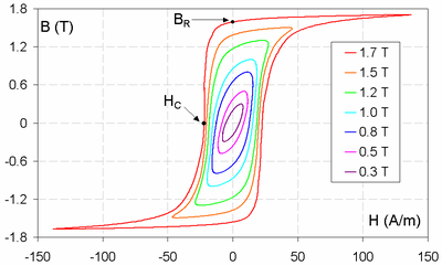
Most importantly, a sufficiently strong magnetic dipole-dipole interaction may lead to their spontaneous ordering, even in the absence of the applied field. This ordering may correspond to either parallel alignment of the dipoles ( ferromagnetism) or anti-parallel alignment of the adjacent dipoles ( antiferromagnetism). Evidently, the external effects of ferromagnetism are stronger, because this phase corresponds to a substantial spontaneous magnetization M even in the absence of an external magnetic field. (The corresponding magnitude of B = 0M is called the remanence field, B R.) The direction of the vector BR may be switched by the application of an external magnetic field, with a magnitude above a certain value H C called coercivity, leading to the well-known hysteretic loops on the [ H, B] plane (see Fig. 14 for a typical example) – similar to those in ferroelectrics, already discussed in Sec. 3.3.
Fig. 5.14. Experimental magnetization
curves of specially processed (cold-rolled)
electrical steel – a solid solution of ~10%
C and ~6% Si in Fe. (Reproduced from
www.thefullwiki.org/Hysteresis under the
Creative Commons BY-SA 3.0 license.)
Just as the ferroelectrics, the ferromagnets may also be hard or soft – in the magnetic rather than mechanical sense. In hard ferromagnets (also called permanent magnets), the dipole interaction is so strong that B stays close to B R in all applied fields below H C, so the hysteretic loops are virtually rectangular. Hence, in lower fields, the magnetization M of a permanent magnet may be considered constant, with the magnitude B R/0. Such hard ferromagnetic materials (notably, rare-earth compounds such as SmCo5, Sm2Co17, and especially Nd2Fe14B), with high remanence fields (~1 T) and high coercivity (~106 A/m), have numerous practical applications.53 Let me give just two, most important examples.
First, permanent magnets are the core components of most electric motors. By the way, this venerable (~150-years-old) technology is currently experiencing a quiet revolution, driven mostly by the electric car development. In the most advanced type of motors, called permanent-magnet synchronous machines (PMSM), the remanence magnetic field B R of a permanent-magnet rotating part of the machine (called the rotor) interacts with the magnetic field of ac currents passed through wire windings in the external, static part of the motor (called the stator). The resulting torque may drive the rotor to extremely high speeds, exceeding 10,000 rotations per minute, enabling the motor to deliver several kilowatts of mechanical power from each kilogram of its mass.
As the second important example, despite the decades of the exponential ( Moore’s-law) progress of semiconductor electronics, most computer data storage systems (e.g., in data centers) are still based 53 Currently, the neodymium-iron-boron compound holds nearly 95% percent of the world permanent-magnet application market, due to its combination of high B R and HC with lower fabrication costs.
Chapter 5
Page 29 of 42
EM: Classical Electrodynamics
on hard disk drives whose active media are submicron-thin layers of hard ferromagnets, with the data bits stored in the form of the direction of the remanent magnetization of small film spots. This technology has reached fantastic sophistication, with the recorded data density of the order of 1012 bits per square inch.54 (Only recently it started to be seriously challenged by solid-state drives based on the floating-gate semiconductor memories already mentioned in Chapter 3.) 55
In contrast, in soft ferromagnets, with their lower magnetic dipole interactions, the magnetization is constant only inside each of the spontaneously formed magnetic domains, while the volume and shape of the domains are affected by the applied magnetic field. As a result, the hysteresis loop’s shape of soft ferromagnets is dependent on the cycled field’s amplitude and cycling history – see Fig. 14. At high fields, their B (and hence M) is driven into saturation, with B B R, but at low fields, they behave essentially as linear magnetics with very high values of m and hence – see the top rows of Table 1.
(The magnetic domain interaction, and hence the low-field susceptibility of such soft ferromagnets are highly dependent on the material’s fabrication technology and its post-fabrication thermal and mechanical treatments.) Due to these high values of , soft ferromagnets, especially iron and its alloys (e.g., various special steels), are extensively used in electrical engineering – for example in the cores of transformers – see the next section.
Due to the relative weakness of the magnetic dipole interaction in some materials, their ferromagnetic ordering may be destroyed by thermal fluctuations, if the temperature is increased above some value called the Curie temperature T C, specific for each material. The transition between the ferromagnetic and paramagnetic phases at T = T C is a classical example of a continuous phase transition, with the average polarization M playing the role of the so-called order parameter that (in the absence of external fields) becomes different from zero only at T < T C, increasing gradually at the further temperature reduction.56
5.6. Systems with magnetic materials
Just as the electrostatics of linear dielectrics, the magnetostatics is very simple in the particular case when all essential stand-alone currents are embedded into a linear magnetic medium with a constant permeability . Indeed, let us assume that we know the solution B0(r) of the magnetic pair of 54 “A magnetic head slider [the read/write head – KKL] flying over a disk surface with a flying height of 25 nm with a relative speed of 20 meters/second [all realistic parameters – KKL] is equivalent to an aircraft flying at a physical spacing of 0.2 µm at 900 kilometers/hour. ” B. Bhushan, as quoted in the (generally good) book by G.
Hadjipanayis, Magnetic Storage Systems Beyond 2000, Springer, 2001.
55 The high-frequency properties of hard ferromagnets are also very non-trivial. For example, according to Eq.
(101), an external magnetic field Bext exerts torque = MBext on the spontaneous magnetic moment M of a unit volume of a ferromagnet. In some nearly-isotropic, mechanically fixed ferromagnetic samples, this torque causes the precession, around the direction of Bext (very similar to that illustrated in Fig. 13), of not the sample as such, but of the magnetization M inside it, with a certain frequency r. If the frequency of an additional ac field becomes very close to r, its absorption sharply increases – the so-called ferromagnetic resonance. Moreover, if
is somewhat higher than r, the effective magnetic permeability () of the material for the ac field may become negative, enabling a series of interesting effects and practical applications. Very unfortunately, I could not find time for their discussion in this series and have to refer the interested reader to literature, for example the monograph by A. Gurevich and G. Melkov, Magnetization Oscillations and Waves, CRC Press, 1996.
56 In this series, a quantitative discussion of such transitions is given in SM Chapter 4.
Chapter 5
Page 30 of 42
EM: Classical Electrodynamics
the genuine (“microscopic”) Maxwell equations (36) in free space, i.e. when the genuine current density j coincides with that of stand-alone currents. Then the macroscopic Maxwell equations (109) and the linear constitutive equation (110) are satisfied with the pair of functions
Hr B0 r
,
Br H
r
B
.
(5.115)
0 r
0
0
Hence the only effect of the complete filling of a fixed-current system with a uniform, linear magnetic medium is the change of the magnetic field B at all points by the same constant factor /0 1
+ m, which may be either larger or smaller than 1. (As a reminder, a similar filling of a system of fixed stand-alone charges with a uniform, linear dielectric always leads to a reduction of the electric field E by a factor of /0 1 + e – the difference whose physics was already discussed at the end of Sec. 4.) However, this simple result is generally invalid in the case of nonuniform (or piecewise-uniform) magnetic samples. To analyze this case, let us first integrate the macroscopic Maxwell equation (107) along a closed contour C limiting a smooth surface S. Now using the Stokes theorem just as at the derivation of Eq. (37), we get the macroscopic version of the Ampère law (37):
Macroscopic
H d I
Ampère
r
.
(5.116)
law
C
Let us apply this relation to a sharp boundary between two regions with different magnetic materials, with no stand-alone currents on the interface, similarly to how this was done for the field E in Sec. 3.4 – see Fig. 3.5. The result is similar as well:
H const
.
(5.117)
On the other hand, the integration of the Maxwell equation (29) over a Gaussian pillbox enclosing a border fragment (again just as shown in Fig. 3.5 for the field D) yields a result similar to Eq. (3.35): B const .
(5.118)
n
For linear magnetic media, with B = H, the latter boundary condition is reduced to H
const
.
(5.119)
n
Let us use these boundary conditions, first of all, to see what happens with a long cylindrical sample of a uniform magnetic material, placed parallel to a uniform external magnetic field B0 – see Fig.
15. Such a sample cannot noticeably disturb the field in the free space outside it, at most of its length: Bext = B0, Hext = 0Bext= 0B0. Now applying Eq. (117) to the dominating surfaces of the sample, we get Hint = H0.57 For a linear magnetic material, these relations yield Bint = Hint = (/0) B0.58 For the high-
media, this means that Bint >> B 0. This effect may be vividly represented as the concentration of the magnetic field lines in high- samples – see Fig. 15 again. (The concentration affects the external field 57 The independence of H on magnetic properties of the sample in this geometry explains why this field’s magnitude is commonly used as the argument in the plots like Fig. 14: such measurements are typically carried out by placing an elongated sample of the material under study into a long solenoid with a controllable current I, so according to Eq. (116), H 0 = nI, regardless of the sample.
58 The reader is highly encouraged to carry out a similar analysis of the fields inside narrow gaps cut in a linear magnetic material, similar to that carried in Sec. 3.3 out for linear dielectrics – see Fig. 3.6 and its discussion.
Chapter 5
Page 31 of 42


Essential Graduate Physics
EM: Classical Electrodynamics
distribution only at distances of the order of (/0) t << l near the sample’s ends.) Such concentration is widely used in such practically important devices as transformers, in which two multi-turn coils are wound on a ring-shaped (e.g., toroidal, see Fig. 6b) core made of a soft ferromagnetic material (such as the transformer steel, see Table 1) with >> 0. This minimizes the number of “stray” field lines, and makes the magnetic flux piercing each wire turn of either coil virtually the same – the equality important for the secondary voltage induction – see the next chapter.
B0
B / B B
0
0
0
t l
~
t l
0
l
Fig. 5. 15. Magnetic field concentration in long, high- magnetic samples (schematically).
Samples of other geometries may create strong perturbations of the external field, extended to distances of the order of the sample’s dimensions. To analyze such problems, we may benefit from a simple, partial differential equation for a scalar function, e.g., the Laplace equation, because in Chapter 2 we have learned how to solve it for many simple geometries. In magnetostatics, the introduction of a scalar potential is generally impossible due to the vortex-like magnetic field lines. However, if there are no stand-alone currents within the region we are interested in, then the macroscopic Maxwell equation (107) for the field H is reduced to H = 0, similar to Eq. (1.28) for the electric field, showing that we may introduce the scalar potential of the magnetic field, m, using a relation similar to Eq. (1.33): H – .
(5.120)
m
Combining it with the homogenous Maxwell equation (29) for the magnetic field, B = 0, and Eq.
(110) for a linear magnetic material, we arrive at a single differential equation, (m) =0. For a uniform medium ((r) = const), it is reduced to our beloved Laplace equation: 2
0 .
(5.121)
m
Moreover, Eqs. (117) and (119) give us very familiar boundary conditions: the first of them
m const ,
(5.122a)
being equivalent to
const ,
(5.122b)
m
while the second one giving
m
const .
(5.123)
n
Indeed, these boundary conditions are absolutely similar for (3.37) and (3.56) of electrostatics, with the replacement .59
59 This similarity may seem strange because earlier we have seen that the parameter is physically more similar to 1/. The reason for this paradox is that in magnetostatics, the magnetic potential m is traditionally used to Chapter 5
Page 32 of 42
EM: Classical Electrodynamics
Let us analyze the geometric effects on magnetization, first using the (too?) familiar structure: a sphere, made of a linear magnetic material, placed into a uniform external field H0 B0/0. Since the differential equation and the boundary conditions are similar to those of the corresponding electrostatics problem (see Fig. 3.11 and its discussion), we can use the above analogy to reuse the solution we already have – see Eqs. (3.63). Just as in the electric case, the field outside the sphere, with 3
R
H r
(5.124)
m
0
cos ,
r R
0
2
2
r
0
is a sum of the uniform external field H0, with the potential – H 0 r cos – H 0 z, and the dipole field (99) with the following induced magnetic dipole moment of the sphere:60
0
3
m 4
R H .
(5.125)
0
20
On the contrary, the internal field is perfectly uniform, and directed along the external one:
3
H
3
B
H
3
H
r cos ,
that
so
,
. (5.126)
m
0
int
0
int
int
r R
0 2
H
2
B
H
2
0
0
0
0
0
0
0
Note that the field Hint inside the sphere is not equal to the applied external field H0. This example shows that the interpretation of H as the “would-be” magnetic field generated by external stand-alone currents j should not be exaggerated by saying that its distribution is independent of the magnetic bodies in the system. In the limit >> 0, Eqs. (126) yield H int/ H 0 << 1, B int/ H 0 = 30, the factor 3 being specific for the particular geometry of the sphere. If a sample is strongly stretched along the applied field, with its length l much larger than the scale t of its cross-section, this geometric effect is gradually decreased, and B int tends to its value H 0 >> B 0, as was discussed above – see Fig. 15.
Now let us calculate the field distribution in a similar, but slightly more complex (and practically important) system: a round cylindrical shell, made of a linear magnetic material, placed into a uniform external field H0 normal to its axis – see Fig. 16.
H
y sin
0
b
H
a
int
0
x cos
Fig. 5.16. Cylindrical magnetic shield.
describe the “would-be field” H, while in electrostatics, the potential describes the actual electric field E. (This tradition persists from the days when H was perceived as a genuine magnetic field.) 60 To derive Eq. (125), we may either calculate the gradient of the m given by Eq. (124), or use the similarity of Eqs. (3.13) and (99), to derive from Eq. (3.17) a similar expression for the magnetic dipole’s potential: 1 m cos
.
m
2
4
r
Now comparing this formula with the second term of Eq. (124), we immediately get Eq. (125).
Chapter 5
Page 33 of 42
EM: Classical Electrodynamics
Since there are no stand-alone currents in the region of our interest, we can again represent the field H(r) by the gradient of the magnetic potential m – see Eq. (120). Inside each of three constant-
regions, i.e. at < b, a < < b, and b < (where is the 2D distance from the cylinder's axis), the potential obeys the Laplace equation (121). In the convenient, polar coordinates (see Fig. 16), we may, guided by the general solution (2.112) of the Laplace equation and our experience in its application to axially-symmetric geometries, look for m in the following form:
H b ' /
b
0
1
cos ,
for
,
(5.127)
m
a b /
a
b
1
1
cos
,
for
,
H cos
,
for a
.
int
Plugging this solution into the boundary conditions (122)-(123) at both interfaces ( = b and
= a), we get the following system of four equations:
H b b ' / b a b b / ,
b
a a b a H a
0
1
1
1
/
1
1
,
int
(5.128)
H b b H a b b
a b a H
0
' / 2
0
1
0
/ 2
1
1
,
/ 2
1
1
,
0
int
for four unknown coefficients a 1, b 1, b 1 ’, and H int. Solving the system, we get, in particular: 2
H
1
int
c
0
(5.129)
H
a b
c
/ ,
with
.
2
c
0
0
According to these formulas, at > 0, the field in the free space inside the cylinder is lower than the external field. This fact allows using such structures, made of high- materials such as permalloy (see Table 1), for passive shielding61 from unintentional magnetic fields (e.g., the Earth's field) – the task very important for the design of many physical experiments. As Eq. (129) shows, the larger is , the closer is c to 1, and the smaller is the ratio H int/ H 0, i.e. the better is the shielding, for the same a/ b ratio. On the other hand, for a given magnetic material, i.e. for a fixed parameter c, the shielding is improved by making the ratio a/ b < 1 smaller, i.e. the shield thicker. On the other hand, as Fig. 16 shows, smaller a leaves less space for the shielded samples, calling for a compromise.
Note that in the limit /0 , both Eq. (126) and Eq. (129), describing different geometries, yield H int/ H 0 0. Indeed, as it follows from Eq. (119), in this limit, the field H tends to zero inside magnetic samples of virtually any geometry. (The formal exception is the longitudinal cylindrical geometry shown in Fig. 15, with t/ l 0, where Hint = H0 for any finite , but even in it, the last equality holds only if t/ l << 0/.)
Now let us discuss a curious (and practically important) approach to systems with relatively thin, closed magnetic cores made of several sections of high- magnetic materials, with the cross-section areas Ak much smaller than the squared lengths lk of the sections – see Fig. 17. If all k >> 0, virtually all field lines are confined to the interior of the core. Then, applying the macroscopic Ampère law (116) to a contour C that follows a magnetic field line inside the core (see, for example, the dashed line in Fig.
17), we get the following approximate expression (exactly valid only in the limit
2
k/0, lk / Ak ):
61 Another approach to the undesirable magnetic fields' reduction is the "active shielding" – the external field’s compensation with the counter-field induced by controlled currents in specially designed wire coils.
Chapter 5
Page 34 of 42


Essential Graduate Physics
EM: Classical Electrodynamics
B
H dl
l H l k NI .
(5.130)
l
k
k
k
C
k
k
k
However, since the magnetic field lines stay in the core, the magnetic flux k BkAk should be the same ( ) for each section, so Bk = / Ak. Plugging this condition into Eq. (130), we get Magnetic
NI
l
Ohm law
k
Φ
,
where
.
(5.131)
k
and
R
R
A
k
k
k
reluctance
k
I
I
C
N
l
N
k
Fig. 5.17. Deriving the “magnetic Ohm law” (131).
k
0
Ak
Note a close analogy of the first of these equations with the usual Ohm law for several resistors connected in series, with the magnetic flux playing the role of electric current, while the product NI, the role of the voltage applied to the chain of resistors. This analogy is fortified by the fact that the second of Eqs. (131) is similar to the expression for the resistance R = l/ A of a long, uniform conductor, with the magnetic permeability playing the role of the electric conductivity . (To sound similar, but still different from the resistance R, the parameter R is called reluctance.) This is why Eq. (131) is called the magnetic Ohm law; it is very useful for approximate analyses of systems like ac transformers, magnetic energy storage systems, etc.
Now let me proceed to a brief discussion of systems with permanent magnets. First of all, using the definition (108) of the field H, we may rewrite the Maxwell equation (29) for the field B as
B
,
(5.132)
0
H M ,0
as
i.e.
H M
While this relation is general, it is especially convenient in permanent magnets, where the magnetization vector M may be approximately considered field-independent.62 In this case, Eq. (132) for H is an exact analog of Eq. (1.27) for E, with the fixed term –M playing the role of the fixed charge density (more exactly, of /0). For the scalar potential m, defined by Eq. (120), this gives the Poisson equation
2 M ,
(5.133)
m
similar to those solved, for quite a few geometries, in the previous chapters.
In the case when M is not only field-independent but also uniform inside a permanent magnet’s volume, then the right-hand sides of Eqs. (132) and (133) vanish both inside the volume and in the 62 Note that in this approximation, there is no difference between the remanence magnetization M R B R/0, of the magnet and its saturation magnetization M S lim H[ B( H)/0 - H].
Chapter 5
Page 35 of 42


Essential Graduate Physics
EM: Classical Electrodynamics
surrounding free space, and give a non-zero effective charge only on the magnet’s surface. Integrating Eq. (132) along a short path normal to the surface and crossing it, we get the following boundary conditions:
H
(5.134)
n
Hn
Hn
M
M cos ,
free
in
space
magnet
in
n
where is the angle between the magnetization vector and the outer normal to the magnet’s surface.
This relation is an exact analog of Eq. (1.24) for the normal component of the field E, with the effective surface charge density (or rather /0) equal to M cos.
This analogy between the magnetic field induced by a fixed, constant magnetization and the electric field induced by surface electric charges enables one to reuse the solutions of quite a few problems considered in Chapters 1-3. Leaving a few such problems for the reader's exercise (see Sec. 7), let me demonstrate the power of this analogy on just two examples specific to magnetic systems. First, let us calculate the force necessary to detach the flat ends of two long, uniform rod magnets, of length l and cross-section area A << l 2, with the saturated remanent magnetization M0 directed along their length – see Fig. 18.
M 0
A
M 0
F
?
min
Fig. 5.18. Detaching two magnets.
l
l
Let us assume we have succeeded in separating the magnets by an infinitesimal distance << A 1/2, l. Then, according to Eqs. (133)-(134), the distribution of the magnetic field near this small gap should be similar to that of the electric field in a system of two equal by opposite surface charges with the surface density proportional to M 0. From Chapters 1-3, we know the properties of such a system very well: within the gap, the field is virtually constant, uniform, proportional to , and independent of
. For its magnitude in the magnetic case, Eq. (134) gives simply H = M 0, and hence B = μ 0 M 0. (Just outside of the gap, the field is very low, because due to the condition A << l 2, the effect of the similar effective charges at the "outer" ends of the rods on the field near the gap t is negligible.) From here, we can readily calculate F min as the force exerted by this field on the effective surface
"charges". However, it is even easier to find it from the following energy argument. Since the magnetic field energy localized inside the magnets and near their outer ends cannot depend on , this small detachment may only alter the energy inside the gap. For this part of the energy, Eq. (57) yields: B 2
M
0
0 2
U
V
A .
(5.135)
2
2
0
0
The gradient of this potential energy is equal to the attraction force F = –( U), trying to reduce Δ U by decreasing the gap, with the following magnitude:
U
2
M A
0
0
F
.
(5.136)
2
The magnet detachment requires an equal and opposite external force. For a typical permanent magnet, with 0 M 0 B R ~ 1T, the force corresponds to a ratio F/ A close to 4105 Pa, a few times the normal atmospheric pressure.
Chapter 5
Page 36 of 42
EM: Classical Electrodynamics
Now let us consider the situation when similar long permanent magnets (such as the magnetic needles used in magnetic compasses) are separated, in otherwise free space, by a larger distance d >> A 1/2 – see Fig. 19. For each needle (Fig. 19a), of a length l >> A 1/2, the right-hand side of Eq. (133) is substantially different from zero only in two relatively small areas at the needle’s ends. Integrating the equation over each area, we see that at distances r >> A 1/2 from each end, we may reduce Eq. (132) to q
m
H
(r r ) (r r )
B q r r r r ,
(5.137)
,
i.e.
m (
)
(
)
0
where r are the ends’ positions, and q m 0 M 0 A, with A being the needle’s cross-section area.63 This expression for B is completely similar to Eq. (3.32) for the electric displacement D, for the particular case of two equal and opposite point charges, i.e. with = q[(r – r+) – (r – r+)], with the only replacement q q m. Since we know the resulting electric field all too well (see, e.g., Eq. (1.7) for E
D/0), we may immediately write a similar expression for the field H:
q
r r
r r
Hr
m
.
(5.138)
4
3
3
0 r r
r r
(a)
(b)
H
q
q
m
m
qm
M
q
0
m
q
q
m
m
Fig. 5.19. (a) “Magnetic charges” at the ends of a thin permanent-magnet needle and (b) the result of its breaking into two parts (schematically).
The resulting magnetic field H(r) exerts on another “magnetic charge” q’ m, located at some point r ’, the force F = q’ mH(r ’).64 Hence if two ends of different needles are separated by an intermediate distance R ( A 1/2 << R << l, see Fig. 19b), we may neglect one term in Eq. (138), and get the following
“magnetic Coulomb law” for the interaction of the nearest ends:
q q'
R
m
m
F
.
(5.139)
4
3
R
0
The “only” (but conceptually, crucial!) difference between this interaction and that of the electric point charges is that the two “magnetic charges” (quasi-monopoles) of a magnetic needle cannot be fully separated. For example, if we break a needle in the middle in an attempt to bring its two ends further apart, two new “point charges” appear – see Fig. 19b.
63 Note that the constant coefficient in the definition of q m, and hence in Eqs. (138)-(139), is the matter of convention. The above choice makes the free-space Maxwell equations D = and B = m (where and m are the volumic densities of the electric and magnetic charges) pleasantly symmetric.
64 This expression is the magnetic analog of the basic equation F = q’ eE(r ’) for the electric charges.
Chapter 5
Page 37 of 42
EM: Classical Electrodynamics
There are several solid-state systems where more flexible structures, similar in their magnetostatics to the needles, may be implemented. First of all, certain (“type-II”) superconductors may carry so-called Abrikosov vortices – flexible tubes with field-suppressed superconductivity inside, each carrying one quantum 0 = / e 210-15 Wb of the magnetic flux. Ending on superconductor’s surfaces, these tubes let their magnetic field lines spread into the surrounding free space, essentially forming magnetic monopole analogs – of course, with equal and opposite “magnetic charges” q m on each end of the tube – just as Fig. 19a shows. Such flux tubes are not only flexible but also stretchable, resulting in several peculiar effects – see Sec. 6.4 for more detail. Another recently found example of such paired quasi-monopoles is spin chains in the so-called spin ices – crystals with paramagnetic ions arranged into a specific (pyrochlore) lattice – such as dysprosium titanate Dy2Ti2O7.65 Let me emphasize again that any reference to magnetic monopoles in such systems should not be taken literally.
In order to complete this section (and this chapter), let me briefly discuss the magnetic field energy U, for the simplest case of systems with linear magnetic materials. In this case, we still may use Eq. (55), but if we want to operate only with macroscopic fields, and hence only stand-alone currents, we should repeat the manipulations that have led us to Eq. (57), using j not from Eq. (35), but from Eq.
(107). As a result, instead of Eq. (57) we get
2
2
B
B
H
Magnetic field
U ur 3
d r, with u
H
,
(5.140) energy:
2
2
2
linear medium
V
This result is evidently similar to Eq. (3.73) of electrostatics.
As a simple but important example of its application, let us again consider a long solenoid (Fig.
6a), but now filled with a linear magnetic material with permeability . Using the macroscopic Ampère law (116), just as we used Eq. (37) for the derivation of Eq. (40), we get
H In , and hence B In
,
(5.141)
where n N/ l, just as in Eq. (40), is the winding density, i.e. the number of wire turns per unit length.
(At = 0, we immediately return to that old result.) Now we may plug Eq. (141) into Eq. (140) to calculate the magnetic energy stored in the solenoid:
2
H
nI 2 lA
U uV
lA
,
(5.142)
2
2
and then use Eq. (72) to calculate its self-inductance:66
U
L
n 2
lA
(5.143)
I 2 / 2
We see that L V, so filling a solenoid with a high- material may allow making it more compact while preserving the same value of inductance. In addition, as the discussion of Fig. 15 has shown, such filling reduces the fringe fields near the solenoid's ends, which may be detrimental for some applications, especially in physical experiments striving for high measurement precision.
65 See, e.g., L. Jaubert and P. Holdworth, J. Phys. – Cond. Matt. 23, 164222 (2011), and references therein.
66 Admittedly, we could get the same result simpler, just by arguing that since the magnetic material fills the whole volume of a substantial magnetic field in this system, the filling simply increases the vector B at all points, and hence its flux , and hence L / I by the factor /0 in comparison with the free-space value (75).
Chapter 5
Page 38 of 42
EM: Classical Electrodynamics
However, we still need to explore the issue of magnetic energy beyond Eq. (140), not only to get a general expression for it in materials with an arbitrary dependence B(H), but also to finally prove Eq.
(54) and explore its relation with Eq. (53). I will do this at the beginning of the next chapter.
5.7. Exercise problems
5.1. DC current I flows around a thin wire loop bent into the form of a plane equilateral triangle with side a. Calculate the magnetic field in the center of the loop.
5.2. A circular wire loop, carrying a fixed dc current, is placed inside a
similar but larger loop, carrying a fixed current in the same direction – see the
figure on the right. Use semi-quantitative arguments to analyze the
I
mechanical stability of the coaxial and coplanar position of the inner loop I'
with respect to its possible angular, axial, and lateral displacements relative to the outer loop.
5.3. Two planar, parallel, long, thin conducting strips of width w, I
separated by distance d, carry equal but oppositely directed currents I – see the figure on the right. Calculate the magnetic field in the plane located in the w
I
middle between the strips, assuming that the flowing currents are uniformly d
distributed across the strip widths.
5.4. For the system studied in the previous problem, but now only in the limit d << w, calculate: (i) the distribution of the magnetic field in space,
(ii) the vector potential of the field,
(iii) the magnetic force (per unit length) exerted on each strip, and
(iv) the magnetic energy and self-inductance of the loop formed by the strips (per unit length).
z
R
d / 2
5.5. Calculate the magnetic field distribution near the center of the system of
I
two similar, plane, round, coaxial wire coils, carrying equal but oppositely directed 0
currents – see the figure on the right.
d / 2
I
z
R
5.6. The two-coil-system considered in the previous problem now carries d / 2
equal and similarly directed currents – see the figure on the right.67 Calculate what I
should be the ratio d/ R for the second derivative 2 B
0
z/ z 2 to equal zero at z = 0.
d / 2
I
67 This Helmholtz coils system, producing a highly uniform field near its center, is broadly used in physical experiment.
Chapter 5
Page 39 of 42
EM: Classical Electrodynamics
j
5.7. DC current of a constant density j flows along a round cylindrical wire of r
R
radius R, with a round cylindrical cavity of radius r cut in it. The cavity’s axis is parallel to that of the wire but offset from it by a distance d < R – r (see the figure on d
0
the right). Calculate the magnetic field inside the cavity.
I
5.8. Calculate the magnetic field’s distribution along the axis of a straight
R
solenoid (see Fig. 6a, partly reproduced on the right) of a finite length l, and a N
l
round cross-section of radius R. Assume that the solenoid has many ( N >> 1, l/ R) I
wire turns, uniformly distributed along its length.
5.9. A thin round disk of radius R, carrying an electric charge of a constant areal density , rotates about its axis with a constant angular velocity . Calculate:
(i) the magnetic field on the disk’s axis,
(ii) the magnetic moment of the disk,
and relate these results.
5.10. A thin spherical shell of radius R, with charge Q uniformly distributed over its surface, rotates about its diameter with a constant angular velocity . Calculate the distribution of the magnetic field everywhere in space.
5.11. A sphere of radius R, made of an insulating material with a uniform electric charge density
, rotates about its diameter with a constant angular velocity . Calculate the magnetic field distribution inside the sphere and outside it.
5.12. A conducting sphere with no total electric charge is rotated about its diameter with a constant angular velocity , in a uniform constant external magnetic field B directed along the rotation axis. Assuming that the sphere’s contribution to the magnetic field is negligibly small, calculate the stationary distribution of the electric charge density inside the sphere and on its surface, and the electrostatic potential both inside and outside the sphere. Quantify the above assumption.
5.13.* The simplest version of the famous homopolar (or “unipolar”)
motor is a thin round conducting disk, placed into a uniform magnetic field B
normal to its plane, with dc current passed between the disk’s center and a
I
sliding electrode (“brush”) on its rim – see the figure on the right.
(i) Express the torque rotating the disk via its radius R, the magnetic
V
field B, and the current I.
I
(ii) If the disk is allowed to rotate about its axis, and the motor is driven by a battery with e.m.f. V, calculate its stationary angular velocity , neglecting friction and the electric circuit’s resistance.
(iii) Now assuming that the current’s path (battery + wires + contacts + disk itself) has a nonzero resistance R, derive and solve the equation for the time evolution of , and analyze the solution.
Chapter 5
Page 40 of 42
EM: Classical Electrodynamics
5.14. The reader is hopefully familiar with the classical Hall effect in the usual rectangular Hall bar geometry – see the left panel of the figure below. However, the effect takes a different form in the so-called Corbino disk – see the right panel of the figure below. (Dark shading shows electrodes, with no appreciable resistance.) Analyze the effect in both geometries, assuming that in both cases, the conductors are thin and planar, have a constant Ohmic conductivity and charge carrier density n, and that the applied magnetic field B is uniform and normal to conductors’ planes.
I
I
I
I
R
B
2
w
R
1
B
l
5.15. A wire with a round cross-section of radius a has been bent into a round loop of radius R
>> a. Prove the formula for its self-inductance, which was mentioned at the end of Sec. 5.3 of the lecture notes: L = 0 R ln( cR/ a), with c ~ 1.
5.16. Prove that:
(i) the self-inductance L of a current loop cannot be negative, and
(ii)any inductance coefficient Lkk’, defined by Eq. (60), cannot be larger than ( LkkLk’k’)1/2.
5.17. Calculate the mutual inductance of two similar thin-wire
h
square-shaped loops offset by distance h in the direction normal to their planes – see the figure on the right.
a
a
5.18.* Estimate the values of magnetic susceptibility due to
(i) orbital diamagnetism, and
(ii) spin paramagnetism,
for a medium with negligible interactions between the induced molecular dipoles. Compare the results.
Hints: For Task (i), you may use the classical model described by Eq. (114) – see Fig. 13. For Task (ii), assume the ordering of spontaneous magnetic dipoles m0, with a fixed magnitude m 0 of the order of the Bohr magneton B, similar to the one sketched for electric dipoles in Fig. 3.7a.
5.19.* Use the classical picture of the orbital (“Larmor”) diamagnetism, discussed in Sec. 5, to calculate its (small) contribution B(0) to the magnetic field B felt by an atomic nucleus, treating the electrons of the atom as a spherically symmetric cloud with an electric charge density ( r). Express the result via the value (0) of the electrostatic potential of the electron cloud, and use this expression for a crude numerical estimate of the ratio B(0)/ B for the hydrogen atom.
5.20. Calculate the self-inductance of a toroidal solenoid
z
I
I
with a round cross-section of radius r ~ R, with N >> 1, R/ r wire r
turns uniformly distributed along the perimeter, and filled with a
linear magnetic material of permeability .
0
R
Chapter 5
Page 41 of 42


Essential Graduate Physics
EM: Classical Electrodynamics
5.21. A long, straight, thin wire carrying current I runs parallel to
I
the plane boundary between two uniform, linear magnetic media – see
1
d
the figure on the right. Calculate the magnetic field everywhere in the system, and the force (per unit length) exerted on the wire.
2
5.22. Solve the magnetic shielding problem similar to that discussed in Sec. 5.6 of the lecture notes, but for a spherical rather than cylindrical shell, with the same central cross-section as shown in Fig. 16. Compare the efficiency of those two shields, for the same shell’s permeability , and the same b/a ratio.
5.23. Calculate the magnetic field’s distribution around a spherical permanent magnet with uniform magnetization M0 = const.
5.24. A limited volume V is filled with a magnetic material with field-independent magnetization M(r). Write explicit expressions for the magnetic field induced by the magnetization and its potential, and recast these expressions into the forms that are more convenient when M(r) = M0 = const throughout the volume.
5.25. Use the results of the previous problem to calculate the
distribution of the magnetic field H along the axis of a straight M
R
0
l
permanent magnet of length 2 l and a round cross-section of radius
l
0
z
R, with a uniform magnetization M
l
0 parallel to the axis – see the
figure on the right.
5.26. A flat end of a long straight permanent magnet, similar to that considered in the previous problem but with an arbitrary cross-section of area A, is stuck to a flat surface of a large sample of a linear magnetic material with a very high permeability >> 0. Calculate the normally directed force needed to detach them.
5.27. A permanent magnet with a uniform magnetization M0 has the form of a spherical shell with an internal radius R 1 and an external radius R 2 > R 1. Calculate the magnetic field inside the shell.
5.28. A very broad film of thickness 2 t is permanently magnetized normally to its plane, with a periodic checkerboard pattern, with the square of area a a:
M
n M , ,
with
,
sgn cos
cos
.
z
x y
M x y
x
y
M 0
z t
a
a
Calculate the magnetic field’s distribution in space.
5.29.* Based on the discussion of the quadrupole electrostatic lens in Sec. 2.4, suggest the permanent-magnet systems that may similarly focus particles moving close to the system’s axis, for the cases when each particle carries:
(i) an electric charge,
(ii) no net electric charge, but a spontaneous magnetic dipole moment m of a certain orientation.
Chapter 5
Page 42 of 42
EM: Classical Electrodynamics
Chapter 6. Electromagnetism
This chapter discusses two major effects that arise when electric and magnetic fields change over time: the “electromagnetic induction” of an additional electric field by changing the magnetic field, and the reciprocal effect of the “displacement currents”– actually, the induction of an additional magnetic field by changing electric field. These two phenomena, which make time-dependent electric and magnetic fields inseparable (hence the term “electromagnetism” 1 ), are reflected in the full system of Maxwell equations, valid for an arbitrary electromagnetic process. On the way toward this system, I will make a brief detour to review the electrodynamics of superconductivity, which (besides its own significance), provides a perfect platform for discussion of the important general issue of gauge invariance.
6.1. Electromagnetic induction
As Eqs. (5.36) show, in static situations (/ t = 0) the Maxwell equations describing the electric and magnetic fields are independent – more exactly, coupled only implicitly, via the continuity equation (4.5) relating their right-hand sides and j. In dynamics, when the fields change in time, the situation is different.
Historically, the first discovered explicit coupling between the electric and magnetic fields was the effect of electromagnetic induction. Although this effect was discovered independently by Joseph Henry, it was a brilliant series of experiments by Michael Faraday, carried out mostly in 1831, that resulted in the first general formulation of the induction law. The summary of Faraday’s numerous experiments has turned out to be very simple: if the magnetic flux defined by Eq. (5.65),
B d 2
Φ
r ,
(6.1)
n
S
through a surface S limited by a closed contour C, changes in time by whatever reason (e.g., either due to a change of the magnetic field B (as in Fig.1), or the contour’s motion, or its deformation, or any combination of the above), it induces an additional, vortex-like electric field Eind directed along the contour – see Fig. 1.
B t
B t
C
C
E
Eind
I
/ R
ind
ind
V
S
S
ind
V
Fig. 6.1. Two simplest ways to observe the Faraday electromagnetic induction.
The exact distribution of Eind in space depends on the system’s details, but its integral along the contour C, called the inductive electromotive force (e.m.f.), obeys a very simple Faraday induction law: 1 It was coined by H. Ørsted in 1820 in the context of his experiments – see the previous chapter.
© K. Likharev
EM: Classical Electrodynamics
d Φ
Faraday
V E d
.
(6.2)
ind
r
ind
induction
dt
C
law
(In the Gaussian units, the right-hand side of this formula has an additional coefficient of 1/ c.) It is straightforward (and hence left for the reader’s exercise) to show that this e.m.f. may be measured, for example, either by inserting a voltmeter into a conducting loop following the contour C or by measuring the small current I = Vind/ R it induces in a thin wire with a sufficiently large Ohmic resistance R,2 whose shape follows that contour – see Fig. 1. (Actually, these methods are not entirely different, because a typical voltmeter measures voltage by the small Ohmic current it drives through the pre-calibrated high internal resistance of the device.) In the context of the latter approach, the minus sign in Eq. (2) may be described by the following Lenz rule: the magnetic field of the induced current I provides a partial compensation of the change of the original flux ( t) with time.3
In order to recast Eq. (2) in a differential form, more convenient in many cases, let us apply to the contour integral in it the Stokes theorem, which was repeatedly used in Chapter 5. The result is V E
.
(6.3)
ind
ind
d 2 r
n
S
Now combining Eqs. (1)-(3), for a contour C whose shape does not change in time (so that the integration along it is interchangeable with the time derivative), we get
B
2
E
.
(6.4)
ind
d r 0
t
S
n
Since the induced electric field is an addition to the gradient field (1.33) created by electric charges, for the net field we may write E = Eind – . However, since the curl of any gradient field is zero,4 () = 0, Eq. (4) remains valid even for the net field E. Since this equation should be correct for any closed area S, we may conclude that
B
Faraday law:
E
0
(6.5)
differential
t
form
at any point. This is the final (time-dependent) form of this Maxwell equation. Superficially, it may look that Eq. (5) is less general than Eq. (2); for example, it does not describe any electric field, and hence any e.m.f. in a moving loop, if the field B is constant in time, even if the magnetic flux (1) through the loop does change in time. However, this is not true; in Chapter 9 we will see that in the reference frame moving with the loop, the e.m.f. does appear.5
2 Such induced current is sometimes called the eddy current, though most often this term is reserved for the distributed currents induced by changing magnetic fields in bulk conductors – see Sec. 3 below.
3 Let me also hope that the reader is familiar with the paradox arising at attempts to measure Vind with a voltmeter without its insertion into the wire loop; if not, I would highly recommend them to solve the offered Problem 2.
4 See, e.g., MA Eq. (11.1).
5 I have to admit that from the beginning of the course, I was carefully sweeping under the rug a very important question: in what exactly reference frame(s) all the equations of electrodynamics are valid? I promise to discuss this issue in detail later in the course (in Chapter 9), and for now would like to get away with a very short answer: all the formulas discussed so far are valid in any inertial reference frame, as defined in classical mechanics – see, e.g., CM Sec. 1.3; however, the fields E and B have to be measured in the same frame.
Chapter 6
Page 2 of 38
EM: Classical Electrodynamics
Now let us reformulate Eq. (5) in terms of the vector potential A. Since the induction effect does not alter the fundamental relation B = 0, we still may represent the magnetic field as prescribed by Eq. (5.27), i.e. as B = × A. Plugging this expression into Eq. (5), and changing the order of the temporal and spatial differentiation, we get
A
E
0 .
(6.6)
t
Hence we can use the same argumentation as in Sec. 1.3 (there applied to the vector E alone) to represent the expression in the parentheses as –, so we get
Fields via
A
E
,
B A .
(6.7)
potentials
t
It is very tempting to interpret the first term of the right-hand side of the expression for E as the one describing the electromagnetic induction alone, and the second term as representing a purely electrostatic field induced by electric charges. However, the separation of these two terms is, to a certain extent, conditional. Indeed, let us consider the gauge transformation already mentioned in Sec. 5.2, A A ,
(6.8)
that, as we already know, does not change the magnetic field. According to Eq. (7), to keep the full electric field intact ( gauge-invariant) as well, the scalar electric potential has to be transformed simultaneously, as
,
(6.9)
t
leaving the choice of an addition to restricted only by the Laplace equation – since the full should satisfy the Poisson equation (1.41) with a gauge-invariant right-hand side. We will return to the discussion of the gauge invariance in Sec. 4.
6.2. Magnetic energy revisited
Now we are sufficiently equipped to revisit the issue of magnetic energy, in particular, to finally prove Eqs. (5.57) and (5.140), and discuss the dichotomy of the signs in Eqs. (5.53) and (5.54). For that, let us consider a sufficiently slow and small magnetic field variation B. If we want to neglect the kinetic energy of the system of electric currents under consideration, as well as the wave radiation effects, we need to prevent its significant acceleration by the arising induction field Eind. Let us suppose that we do this by virtual balancing of this field by an external electric field Eext = –Eind. According to Eq. (4.38), the work of that field6 on the stand-alone currents of the system during a small time interval
t, and hence the change of the potential energy of the system, is U
δt jE d 3 r,
that
so
j E
,
(6.10)
ext
U δt d 3 r
ind
V
V
6 As a reminder, the magnetic component of the Lorentz force (5.10), vB, is always perpendicular to the particle velocity v, so the magnetic field B itself cannot perform any work on moving charges, i.e. on currents.
Chapter 6
Page 3 of 38
EM: Classical Electrodynamics
where the integral is over the volume of the system. Now expressing the current density j from the macroscopic Maxwell equation (5.107), j = H, and then applying the vector algebra identity7
HE H
,
(6.11)
ind
Eind E H
ind
we get
U
δt H E d 3 r δt E H
d 3 r .
(6.12)
V
V
According to the divergence theorem, the second integral in the right-hand of this equality is equal to the flux of the so-called Poynting vector S E H through the surface limiting the considered volume V. Later in the course we will see that this flux represents, in particular, the power of electromagnetic radiation through the surface. If such radiation is negligible (as it always is if the field variation is sufficiently slow), the surface may be selected sufficiently far, so that the flux of S vanishes.
In this case, we may express E from the Faraday induction law (5) to get
B
U
δt H d 3 r H B
d 3 r .
(6.13)
t
V
V
Just as in the electrostatics (see Eqs. (1.65) and (3.73), and their discussion), this relation may be interpreted as the variation of the magnetic field energy U of the system, and represented in the form Magnetic
U
u
r d 3 r,
with u H δB
.
(6.14) energy’s
variation
V
This is a keystone result; let us discuss it in some detail.
First of all, for a system filled with a linear and isotropic magnetic material, we may use Eq. (14) together with Eq. (5.110): B = H. Integrating the result over the variation of the field from 0 to a certain final value B, we get Eq. (5.140) – so important that it deserves rewriting again: 2
B
U u 3
d r, with u
r
.
(6.15)
2
V
In the simplest case of free space (no magnetics at all, so j above is the complete current density), we may take = 0, and reduce Eq. (15) to Eq. (5.57). Now performing backward the transformations that took us, in Sec. 5.3, to derive that relation from Eq. (5.54), we finally have the latter formula proved – as was promised in the last chapter.
It is very important, however, to understand the limitations of Eq. (15). For example, let us try to apply it to a very simple problem, which was already analyzed in Sec. 5.6 (see Fig. 5.15): a very long cylindrical sample of a linear magnetic material placed into a fixed external field Hext parallel to the sample’s length. It is evident that in this simple geometry, the field H and hence the field B = H have to be uniform inside the sample, besides negligible regions near its ends, so Eq. (15) is reduced to B 2
U
V ,
(6.16)
2
7 See, e.g., MA Eq. (11.7) with f = Eind and g = H.
Chapter 6
Page 4 of 38
EM: Classical Electrodynamics
where V = Al is the cylinder’s volume. Now if we try to calculate the static (equilibrium) value of the field from the minimum of this potential energy, we get evident nonsense: B = 0 (WRONG!).8
The situation may be readily rectified by using the notion of the Gibbs potential energy, just as it was done for the electric field in Sec. 3.5 (and implicitly in the end of Sec. 1.3). According to Eq. (14), in magnetostatics, the Cartesian components of the field H(r) play the role of the generalized forces, while those of the field B(r), of the generalized coordinates (per unit volume).9 As the result, the Gibbs potential energy, whose minimum corresponds to the stable equilibrium of the system under the effect of a fixed generalized force (in our current case, of the fixed external field Hext), is
Gibbs
potential
U u
d r,
with u
u
,
(6.17)
G
r 3
G
G r
r H rBr
ext
energy
V
– the expression parallel to Eq. (3.78). For a system with linear magnetics, we may use, for the energy density u(r), our result (15), getting the following Gibbs energy’s density: 1
1
u (r)
B B H
B
B H
,
(6.18)
G
ext
ext 2
const
2
2
where “const” means a term independent of the field B inside the sample. For our simple cylindrical system, with its uniform fields, Eqs. (17)-(18) gives the following full Gibbs energy of the sample:
B H
int
ext 2
U
V const ,
(6.19)
G
2
whose minimum immediately gives the correct stationary value Bint = Hext, i.e. Hint Bint/ = Hext, which was already obtained in Sec. 5.6 in a different way, from the boundary condition (5.117).
Now notice that with this result on hand, Eq. (18) may be rewritten in a different form: 1
2
B
B
u (r)
B B
B
,
(6.20)
G
2
2
similar to Eq. (15) for u(r), but with an opposite sign. This sign dichotomy explains that of Eqs. (5.53) and Eq. (5.54); indeed, as was already noted in Sec. 5.3, the former of these expressions gives the potential energy whose minimum corresponds to the equilibrium of a system with fixed currents. (In our current example, these are the external stand-alone currents inducing the field Hext.) So, the energy Uj given by Eq. (5.53) is essentially the Gibbs energy U G defined by Eqs. (17) and (for the equilibrium state of linear magnetic media) by Eq. (20), while Eq. (5.54) is just another form of Eq. (15) – as was explicitly shown in Sec. 5.3.10
8 This erroneous result cannot be corrected by just adding the energy of the field outside the cylinder because in the limit A 0, this field is not affected by the internal field B.
9 Note an aspect in that the analogy with electrostatics is not quite complete. Indeed, according to Eq. (3.76), in electrostatics, the role of a generalized coordinate is played by the “would-be” field D, and that of the generalized force, by the actual (if macroscopic) electric field E. This difference may be traced back to the fact that the electric field E may perform work on a moving charged particle, while the magnetic field cannot. However, this difference does not affect the full analogy of the expressions (3.73) and (15) for the field energy density in linear media.
10 As was already noted in Sec. 5.4, one more example of the energy Uj (i.e. U G) is given by Eq. (5.100).
Chapter 6
Page 5 of 38
EM: Classical Electrodynamics
Let me complete this section by stating that the difference between the energies U and U G is not properly emphasized (or even left obscure) in some textbooks, so the reader is advised to get additional clarity by solving a few additional simple problems – for example, by spelling out these energies for a long straight solenoid (Fig. 5.6a), and then using the results to calculate the pressure exerted by the magnetic field on the solenoid’s walls (windings) and the longitudinal forces exerted on its ends.
6.3. Quasistatic approximation and skin effect
Perhaps the most surprising experimental fact concerning the time-dependent electromagnetic phenomena is that unless they are so fast that one more new effect of the displacement currents (to be discussed in Sec. 7 below) becomes noticeable, all formulas of electrostatics and magnetostatics remain valid, with the only exception: the generalization of Eq. (3.36) to Eq. (5), describing the Faraday induction. As a result, the system of macroscopic Maxwell equations (5.109) is generalized to
B
E
0,
H j,
Quasistatic
t
(6.21) approximation
D ,
B 0.
(As it follows from the discussions in chapters 3 and 5, the corresponding system of microscopic Maxwell equations for the genuine, “microscopic” fields E and B may be obtained from Eq. (21) by the formal substitutions D = 0E and H = B/0, and the replacement of the stand-alone charge and current densities and j with their full densities.11) These equations, whose range of validity will be quantified in Sec. 7, define the so-called quasistatic approximation of electromagnetism and are sufficient for an adequate description of a broad range of physical effects.
In order to form a complete system of equations, Eqs. (21) should be augmented by constituent equations describing the medium under consideration. For a linear isotropic material, they may be taken in the simplest (and simultaneously, most common) linear and isotropic forms already discussed in Chapters 4 and 5:
j E
,
B H
.
(6.22)
If the conductor is uniform, i.e. the coefficients and are constant inside it, the whole system of Eqs.
(21)-(22) may be reduced to just one simple equation. Indeed, a sequential substitution of these equations into each other, using a well-known vector-algebra identity12 in the middle, yields: B
1
1
1
1
E j ( H)
( B)
(B) 2
B
t
(6.23)
1
2
B.
Thus we have arrived, without any further assumptions, at a rather simple partial differential equation. Let us use it for an analysis of the so-called skin effect, the phenomenon of an Ohmic conductor’s self-shielding from the alternating ( ac) magnetic field. In its simplest geometry (Fig. 2a), an 11 Obviously, in free space, the last replacement is unnecessary, because all charges and currents may be treated as
“stand-alone” ones.
12 See, e.g., MA Eq. (11.3).
Chapter 6
Page 6 of 38


Essential Graduate Physics
EM: Classical Electrodynamics
external source (which, at this point, does not need to be specified) produces, near a plane surface of a bulk conductor, a spatially-uniform ac magnetic field H(0)( t) parallel to the surface.13
y
(a)
(b)
0
,
C
C
1
2
0
Fig. 6.2. (a) The skin effect in
0
the simplest, planar geometry,
H 0
H
H 0
(0)
H
and (b) two Ampère contours,
H x
C 1 and C 2, for deriving the
n
J
“macroscopic” ( C 1) and the
0
x
“coarse-grain” ( C 2) boundary
s
s
conditions for H.
Selecting the coordinate system as shown in Fig. 2a, we may express this condition as
0
H
H
t
( n
)
.
(6.24)
x 0
y
The translational symmetry of our simple problem within the surface plane [ y, z] implies that inside the conductor, / y = / z = 0 as well, and H = H( x, t)n y even at x 0, so Eq. (23) for the conductor’s interior is reduced to a differential equation for just one scalar function H( x, t) = B( x, t)/:
H
1
2
H
,
for x 0 .
(6.25)
2
t
x
This equation may be further simplified by noticing that due to its linearity, we may use the linear superposition principle for the time dependence of the field,14 via expanding it, as well as the external field (24), into the Fourier series:
H ( x, t) H ( x)
e i t
, for . x ,0
(6.26)
0
0
H ( t)
H e i t ,
for
x ,
0
and arguing that if we know the solution for each frequency component of the series, the whole field may be found through the straightforward summation (26) of these solutions.
For each single-frequency component, Eq. (25) is immediately reduced to an ordinary differential equation for the complex amplitude H( x):15
13 Due to the simple linear relation B = H between the fields B and H, it does not matter too much which of them is used for the solution of this problem, with a slight preference for H, due to the simplicity of Eq. (5.117) –
the only boundary condition relevant for this simple geometry.
14 Another way to exploit the linearity of Eq. (6.25) is to use the spatial-temporal Green’s function approach to explore the dependence of its solutions on various initial conditions. Unfortunately, because of a lack of time, I have to leave an analysis of this opportunity for the reader’s exercise.
15 Let me hope that the reader is not intimidated by the (very convenient) use of such complex variables for describing real fields; their imaginary parts always disappear at the final summation (26). For example, if the Chapter 6
Page 7 of 38
EM: Classical Electrodynamics
d 2
1
i H
H .
(6.27)
2
dx
From the theory of linear ordinary differential equations, we know that Eq. (27) has the following general solution:
x
x
H ( x
H e H e
)
,
(6.28)
where the constants are the roots of the characteristic equation that may be obtained by the substitution of any of these two exponents into the initial differential equation. For our particular case, the characteristic equation following from Eq. (27) is simply
2
i
(6.29)
and its roots are, obviously,
1 i
.
(6.30)
i 1/2
1/2
2
For our problem, the field cannot grow exponentially at x +, so only one of the coefficients, namely the H– corresponding to the decaying exponent, with Re – < 0, may be different from zero, i.e.
H( x) = H(0)exp{ –x}. To find the constant factor H(0), we can integrate the macroscopic Maxwell equation H = j along a pre-surface contour – say, the contour C 1 shown in Fig. 2b. The right-hand side’s integral is negligible because the stand-alone current density j does not include the “genuinely-surface” currents responsible for the magnetic permeability – see Fig. 5.12. As a result, we get the boundary condition similar to Eq. (5.117) for the stationary magnetic field: H = const at x = 0, giving us
H ,
0 t
0
H t,
i.e. H
0
0
H ,
(6.31)
so the final solution of our boundary problem may be represented as
0
0
x
x
H ( x) H
exp x
H
exp
exp
i t
,
(6.32)
s
s
where the constant s, with the dimension of length, is called the skin depth: 1/ 2
1
2
.
(6.33)
Skin
s
Re
depth
This solution describes the skin effect: the penetration of the ac magnetic field, and the eddy currents j, into a conductor only to a finite depth of the order of s. Let me give a few numerical examples of this depth: for copper at room temperature, s 1 cm at the usual ac power distribution frequency of 60 Hz, and is of the order of just 1 m at a few GHz, i.e. at typical frequencies of cell phone signals and kitchen microwave magnetrons. On the other hand, for lightly salted water, s is close to 250 m at just 1 Hz (with significant implications for radio communications with submarines), and of external field is purely sinusoidal, with the actual (positive) frequency , each sum in Eq. (26) has just two terms, with complex amplitudes H and H- = H*, so their sum is always real. (For a more detailed discussion of this issue, see, e.g., CM Sec. 5.1.)
Chapter 6
Page 8 of 38
EM: Classical Electrodynamics
the order of 1 cm at a few GHz (explaining, in particular, the nonuniform heating of a soup bowl in a microwave oven).16
Let me hope that the equality chain (23) makes the physics of this effect very clear: the external electric field E, which is Faraday-induced by an external ac magnetic field, drives the eddy currents j, which in turn induce their own magnetic field that eventually (at x ~ s) compensates the external one.
Let us quantify these E and j. Since we have used, in particular, relations j = H = × B/, and E =
j/, and spatial differentiation of an exponent yields a similar exponent, the electric field and current density have the same spatial dependence as the magnetic field, i.e. penetrate the conductor only by distances of the order of s(). Their vectors are directed normally to B, while still being parallel to the conductor’s surface:17
j
x
H ( x) n ,
E x
H ( x)n
.
(6.34)
z
z
We may use these expressions, in particular, to calculate the time-averaged power density (4.39) of the energy dissipation, for the important case of a sinusoidal (“monochromatic”) field H( x, t) = H( x)
cos( t + ), and hence sinusoidal eddy currents: j( x, t) = j( x) cos( t + ’): 2
2
j x, t
j x cos t
2
2
'
j x
2
2
2
H x
H x
p x
.
(6.35)
2
2
2
s
Now the (elementary) integration of this expression along the x-axis (through all the skin depth), using the exponential law (6.32), gives us the following average power of the energy loss per unit area: Energy
loss
d
P
1
2
at skin
p x
0
s
2
0
dx
H
H
.
(6.36)
effect
dA
2
4
0
s
We will extensively use this expression in the next chapter to calculate the energy losses in microwave waveguides and resonators with conducting (practically, metallic) walls, and for now let me note only that according to Eqs. (33) and (36), for a fixed magnetic field amplitude, the losses grow with frequency as 1/2.
One more important remark concerning Eqs. (34): integrating the first of them over x, with the help of Eq. (32), we may see that the linear density J of the surface currents (measured in A/m), is simply and fundamentally related to the applied magnetic field:
J j
x
0
dx
H n
.
(6.37)
z
0
Since this relation does not have any frequency-dependent factors, we may sum it up for all frequency components, and get a universal relation
J t
0
H t
0
n H
0
0
,
(6.38a)
z
t n n
y
x
H t n x
H t n
16 Let me hope that the reader’s physical intuition makes it evident that the skin effect remains conceptually the same for samples of any shape, besides possibly some quantitative details of the field distribution.
17 The loop (vortex) character of the induced current lines, responsible for the term “eddy”, is not very apparent in the 1D geometry explored above, with the near-surface currents (Fig. 2b) looping only implicitly, at z .
Chapter 6
Page 9 of 38
EM: Classical Electrodynamics
(where n = –n x is the outer normal to the surface – see Fig. 2b) or, in a different form, Coarse-grain
H
t n J( t),
(6.38b) boundary
relation
where H is the full change of the field through the skin layer. This simple coarse-grain relation (independent of the choice of coordinate axes), is also independent of the used constituent relations (22), and is by no means occasional. Indeed, it may be readily obtained from the macroscopic Ampère law (5.116), by applying it to a contour drawn around a fragment of the surface, extending under it substantially deeper than the skin depth – see the contour C 2 in Fig. 2b. Hence, Eq. (38) is valid regardless of the exact law of the field penetration.
For the skin effect, this fundamental relationship between the linear current density and the external magnetic field implies that the skin effect’s implementation does not necessarily require a dedicated ac magnetic field source. For example, the effect takes place in any wire that carries an ac current, leading to a current’s concentration in a surface sheet of thickness ~s. (Of course, the quantitative analysis of this problem in a wire with an arbitrary cross-section may be technically complicated, because it requires solving Eq. (23) for the corresponding 2D geometry; even for the round cross-section, the solution involves the Bessel functions.) In this case, the ac magnetic field outside the conductor, which still obeys Eq. (38), may be better interpreted as the effect, rather than the cause, of the ac current flow.
Finally, please mind the limited validity of all the above results. First, for the quasistatic approximation to be valid, the field frequency should not be too high, so the displacement current effects are negligible. (Again, this condition will be quantified in Sec. 7 below; it will show that for metals, the condition is violated only at extremely high frequencies above ~1018 s-1.) A more practical upper limit on is that the skin depth s should stay much larger than the mean free path l of charge carriers , 18 because beyond this point, the constituent relation between the vectors j(r) and E(r) becomes essentially non-local. Both theory and experiment show that at s below l, the skin effect persists, but acquires a frequency dependence slightly different from Eq. (33): s –1/3 rather than –1/2.
Historically, this anomalous skin effect has been very useful for the measurements of the Fermi surfaces of metals.19
6.4. Electrodynamics of superconductivity, and the gauge invariance
The effect of superconductivity20 takes place (in certain materials only, mostly metals) when temperature T is reduced below a certain critical temperature T c specific for each material. For most metallic superconductors, T c is of the order of typically a few kelvins, though several compounds (the so-called high-temperature superconductors) with T c above 100 K have been found since 1987. The most notable property of superconductors is the absence, at T < T c, of measurable resistance to (not very high) dc currents. However, the electromagnetic properties of superconductors cannot be described by just taking = in our previous results. Indeed, for this case, Eq. (33) would give s = 0, i.e., no ac 18 A discussion of the mean free path may be found, for example, in SM Chapter 6. In very clean metals at very low temperatures, s may approach l at frequencies as low as ~1 GHz, but at room temperature, the crossover between the normal to the anomalous skin effect takes place only at ~ 100 GHz.
19 See, e.g., A. Abrikosov, Introduction to the Theory of Normal Metals, Academic Press, 1972.
20 Discovered experimentally in 1911 by Heike Kamerlingh Onnes.
Chapter 6
Page 10 of 38
EM: Classical Electrodynamics
magnetic field penetration at all. Experiment shows something substantially different: weak magnetic fields do penetrate into superconductors by a material-specific distance L ~ 10-7-10-6 m, the so-called London’s penetration depth,21 which is virtually frequency-independent until the skin depth s, of the same material in its “normal” state, i.e. the absence of superconductivity, becomes less than L. (This crossover happens typically at frequencies ~ 1013-1014 s-1.) The smallness of L on the human scale means that the magnetic field is pushed out from macroscopic samples at their transition into the superconducting state.
This Meissner-Ochsenfeld effect, discovered experimentally in 1933,22 may be partly understood using the following classical reasoning. Our discussion of the Ohm law in Sec. 4.2 implied that the current’s (and hence the electric field’s) frequency is either zero or sufficiently low. In the classical Drude reasoning, this is acceptable while << 1, where is the effective carrier scattering time participating in Eqs. (4.12)-(4.13). If this condition is not satisfied, we should take into account the charge carrier inertia; moreover, in the opposite limit >> 1, we may neglect the scattering at all.
Classically, we can describe the charge carriers in such a “perfect conductor” as particles with a nonzero mass m, which are accelerated by the electric field following the 2nd Newton law (4.11), v
m F E
q ,
(6.39)
so the current density j = qnv that they create, changes in time as q 2 n
j
v
qn
E .
(6.40)
m
In terms of the Fourier amplitudes of the functions j( t) and E( t), this means q 2 n
i
j
E .
(6.41)
m
Comparing this formula with the relation j = E implied in the last section, we see that we can use all its results with the following replacement:
q 2 n
i
.
(6.42)
m
This change replaces the characteristic equation (29) with
2
m
q 2
2
n
i
,
i.e.
,
(6.43)
iq 2 n
m
i.e. replaces the skin effect with the field penetration by the following frequency-independent depth: 1/ 2
1
m
.
(6.44)
2
q
n
Superficially, this means that the field decay into the superconductor does not depend on frequency: 21 Named so to acknowledge the pioneering theoretical work of brothers Fritz and Heinz London – see below.
22 It is hardly fair to shorten this name to just the “Meissner effect” as it is frequently done, because of the reportedly crucial contribution by Robert Ochsenfeld, then a Walther Meissner’s student, to the discovery.
Chapter 6
Page 11 of 38
EM: Classical Electrodynamics
x /
H ( x, t) H ( ,
0 t) e
,
(6.45)
thus explaining the Meissner-Ochsenfeld effect.
However, there are two problems with this result. First, for the parameters typical for good metals ( q = – e, n ~ 1029 m-3, m ~ m e, 0), Eq. (44) gives ~ 10-8 m, one or two orders of magnitude lower than the experimental values of L. Experiment also shows that the penetration depth diverges at T
T c, which is not predicted by Eq. (44).
The second, much more fundamental problem with Eq. (44) is that it has been derived for
>> 1. Even if we assume that somehow there is no scattering at all, i.e. = , at 0 both parts of the characteristic equation (43) vanish, and we cannot make any conclusion about . This is not just a mathematical artifact we could ignore. For example, let us place a non-magnetic metal into a static external magnetic field at T > T c. The field would completely penetrate the sample. Now let us cool it.
As soon as the temperature is decreased below T c, the above calculations would become valid, forbidding the penetration into the superconductor of any change of the field, so the initial field would be “frozen” inside the sample. The Meissner-Ochsenfeld experiments have shown something completely different: as T is lowered below T c, the initial field is being expelled out of the sample.
The resolution of these contradictions is provided by quantum mechanics. As was explained in 1957 in a seminal work by J. Bardeen, L. Cooper, and J. Schrieffer (commonly referred to as the BCS
theory), superconductivity is due to the correlated motion of electron pairs, with opposite spins and nearly opposite momenta. Such Cooper pairs, each with the electric charge q = –2 e and zero spin, may form only in a narrow energy layer near the Fermi surface, of a certain thickness ( T). This parameter
( T), which may be also interpreted as the binding energy of the pair, tends to zero at T T c, while at T
<< T c it has a virtually constant value (0) 3.5 k B T c, of the order of a few meV for most superconductors. This fact readily explains the relatively low spatial density of the Cooper pairs: n p ~
n( T)/F ~ 1026 m-3. With the correction n n p, Eq. (44) for the penetration depth becomes 1/ 2
m
London’s
.
(6.46) penetration
L
2
q
n
depth
p
This result diverges at T T c, and generally fits the experimental data reasonably well, at least for the so-called “clean” superconductors with the mean free path l = v F (where v F ~ (2 mF)1/2 is the r.m.s.
velocity of electrons on the Fermi surface) much longer than the Cooper pair size – see below.
The smallness of the coupling energy ( T) is also a key factor in the explanation of the Meissner-Ochsenfeld effect. Because of Heisenberg’s quantum uncertainty relation r p ~ , the spatial extension of the Cooper-pair’s wavefunction (the so-called coherence length of the superconductor) is relatively large: ~ r ~ / p ~ v F/( T) ~ 10-6 m. As a result, n p3 >> 1, meaning that the wavefunctions of the pairs are strongly overlapped in space. Due to their integer spin, Cooper pairs behave like bosons, which means in particular that at low temperatures they exhibit the so-called Bose-Einstein condensation onto the same ground energy level g.23 This means that the quantum frequency
23 A quantitative discussion of the Bose-Einstein condensation of bosons may be found in SM Sec. 3.4, though the full theory of superconductivity is more complicated because it has to describe the condensation taking place simultaneously with the formation of effective bosons (Cooper pairs) from fermions (single electrons). For a Chapter 6
Page 12 of 38