DSPA by Douglas Jones, Don Johnson, et al - HTML preview
Download the book in PDF, ePub for a complete version.
V=ℂ N , =ℂ
,
sequences in " lp "
=ℂ
functions in " ℒp "
, =ℂ
where we have assumed the usual definitions of addition and multiplication. From now on, we will
denote the arbitrary vector space ( V, , +, ⋅) by the shorthand V and assume the usual selection of
( , +, ⋅). We will also suppress the "⋅" in scalar multiplication, so that ( α ⋅ x) becomes αx .
A subspace of V is a subset M⊂ V for which
1. x+y∈ M , x∈ M∧y∈ M
2. αx∈ M , x∈ M∧ α∈
Note that every subspace must contain 0, and that V is a subspace of itself.


The span of set S⊂ V is the subspace of V containing all linear combinations of vectors in S.
When
,
A subset of linearly-independent vectors
is called a basis for V when its span
equals V. In such a case, we say that V has dimension N. We say that V is infinite-dimensional
[6] if it contains an infinite number of linearly independent vectors.
V is a direct sum of two subspaces M and N, written V=( M⊕ N) , iff every x∈ V has a unique representation x=m+n for m∈ M and n∈ N .
Note that this requires M⋂ N={0}
Normed Vector Space*
Now we equip a vector space V with a notion of "size".
A norm is a function ( (∥⋅∥ : V→ℝ) ) such that the following properties hold (
, x∈ V∧y∈ V and , α∈ ):
1. ∥x∥≥0 with equality iff x=0
2. ∥ αx∥=| α|⋅∥x∥
3. ∥x+y∥≤∥x∥+∥y∥ , (the triangle inequality).
In simple terms, the norm measures the size of a vector. Adding the norm operation to a vector
space yields a normed vector space. Important example include:
1. V=ℝ N ,
2. V=ℂ N ,
3. V= lp ,
4. V= ℒp ,


Inner Product Space*
Next we equip a normed vector space V with a notion of "direction".
An inner product is a function ( (< ·, ·> : V× V)→ℂ ) such that the following properties hold (
, x∈ V∧y∈ V∧z∈ V and , α∈ ):
1.
2. < x, αy>= α< x, y> ...implying that
3. < x, y+z>=< x, y>+< x, z>
4. < x, x>≥0 with equality iff x=0
In simple terms, the inner product measures the relative alignment between two vectors.
Adding an inner product operation to a vector space yields an inner product space. Important
examples include:
1. V=ℝ N , (< x, y> ≔ xTy)
2. V=ℂ N , (< x, y> ≔ xHy)
3. V= l 2 ,
4. V= ℒ 2 ,
The inner products above are the "usual" choices for those spaces.
The inner product naturally defines a norm:
though not every norm can be
defined from an inner product. [7] Thus, an inner product space can be considered as a normed
vector space with additional structure. Assume, from now on, that we adopt the inner-product
norm when given a choice.
The Cauchy-Schwarz inequality says
|< x, y>|≤∥x∥∥y∥ with equality iff ∃, α∈ :(x= αy) .
When < x, y>∈ℝ , the inner product can be used to define an "angle" between vectors:
Vectors x and y are said to be orthogonal, denoted as (x ⊥ y) , when < x, y>=0 . The Pythagorean theorem says: (∥x+y∥)2=(∥x∥)2+(∥y∥)2 , (x ⊥ y) Vectors x and y are said to


be orthonormal when (x ⊥ y) and ∥x∥=∥y∥=1 .
(x ⊥ S) means (x ⊥ y) for all y∈ S . S is an orthogonal set if (x ⊥ y) for all x∧y∈ S s.t. x≠y . An orthogonal set S is an orthonormal set if ∥x∥=1 for all x∈ S . Some examples of orthonormal
sets are
1. ℝ3 :
2. ℂ N : Subsets of columns from unitary matrices
3. l 2 : Subsets of shifted Kronecker delta functions S⊂{{ δ[ n− k]}| k∈ℤ}
4. ℒ 2 :
for unit pulse f( t)= u( t)− u( t− T) , unit step u( t)
where in each case we assume the usual inner product.
Hilbert Spaces*
Now we consider inner product spaces with nice convergence properties that allow us to define
countably-infinite orthonormal bases.
A Hilbert space is a complete inner product space. A complete [8] space is one where all Cauchy sequences converge to some vector within the space. For sequence { xn} to be Cauchy,
the distance between its elements must eventually become arbitrarily small:
For a sequence { xn} to be convergent to x, the distance
between its elements and x must eventually become arbitrarily small:
Examples are listed below (assuming the usual inner products):
1. V=ℝ N
2. V=ℂ N
3. V= l 2 ( i.e. , square summable sequences)
4. V= ℒ 2 ( i.e. , square integrable functions)
We will always deal with separable Hilbert spaces, which are those that have a countable [9]
orthonormal (ON) basis. A countable orthonormal basis for V is a countable orthonormal set
such that every vector in V can be represented as a linear combination of elements in S:
Due to the orthonormality of S, the basis coefficients are given by


We can see this via:
where
(where the second equality invokes the continuity of the inner product). In finite n-dimensional
spaces ( e.g. , ℝ n or ℂ n ), any n-element ON set constitutes an ON basis. In infinite-dimensional
spaces, we have the following equivalences:
1.
is an ON basis
2. If
for all i, then y=0
3.
(Parseval's theorem)
4. Every y∈ V is a limit of a sequence of vectors in
Examples of countable ON bases for various Hilbert spaces include:
1. ℝ n :
for
with "1" in the i th position
2. ℂ n : same as ℝ n
3. l 2 :
, for ({ δi[ n]} ≔ { δ[ n− i]}) (all shifts of the Kronecker sequence)
4. ℒ 2 : to be constructed using wavelets ...
Say S is a subspace of Hilbert space V. The orthogonal complement of S in V, denoted S⊥ , is
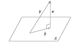
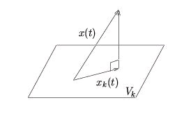
the subspace defined by the set {x∈ V|(x ⊥ S)} . When S is closed, we can write V=( S⊕ S⊥) The orthogonal projection of y onto S, where S is a closed subspace of V, is
s.t.
is an ON basis for S. Orthogonal projection yields the best approximation of y in S:
The approximation error
obeys the orthogonality principle:
(e ⊥ S) We illustrate this concept using V=ℝ3 (Figure 4.10) but stress that the same geometrical interpretation applies to any Hilbert space.
Figure 4.10.


A proof of the orthogonality principle is:
()
4.3. Discrete Wavelet Transform
Discrete Wavelet Transform: Main Concepts*
Main Concepts
The discrete wavelet transform (DWT) is a representation of a signal x( t)∈ ℒ 2 using an
orthonormal basis consisting of a countably-infinite set of wavelets. Denoting the wavelet basis as
, the DWT transform pair is
()
()
where { d k , n } are the wavelet coefficients. Note the relationship to Fourier series and to the
sampling theorem: in both cases we can perfectly describe a continuous-time signal x( t) using a
countably-infinite ( i.e. , discrete) set of coefficients. Specifically, Fourier series enabled us to
describe periodic signals using Fourier coefficients { X[ k]| k∈ℤ} , while the sampling theorem
enabled us to describe bandlimited signals using signal samples { x[ n]| n∈ℤ} . In both cases,
signals within a limited class are represented using a coefficient set with a single countable index.
The DWT can describe any signal in ℒ 2 using a coefficient set parameterized by two countable
indices:
.
Wavelets are orthonormal functions in ℒ 2 obtained by shifting and stretching a mother wavelet,
ψ( t)∈ ℒ 2 . For example,


()
defines a family of wavelets
related by power-of-two stretches. As k increases,
the wavelet stretches by a factor of two; as n increases, the wavelet shifts right.
When ∥ ψ( t)∥=1 , the normalization ensures that ∥ ψ k , n ( t)∥=1 for all k∈ℤ , n∈ℤ .
Power-of-two stretching is a convenient, though somewhat arbitrary, choice. In our treatment of
the discrete wavelet transform, however, we will focus on this choice. Even with power-of two
stretches, there are various possibilities for ψ( t) , each giving a different flavor of DWT.
Wavelets are constructed so that
( i.e. , the set of all shifted wavelets at fixed scale k),
describes a particular level of 'detail' in the signal. As k becomes smaller ( i.e. , closer to –∞ ), the
wavelets become more "fine grained" and the level of detail increases. In this way, the DWT can
give a multi-resolution description of a signal, very useful in analyzing "real-world" signals.
Essentially, the DWT gives us a discrete multi-resolution description of a continuous-time
signal in ℒ 2 .
In the modules that follow, these DWT concepts will be developed "from scratch" using Hilbert
space principles. To aid the development, we make use of the so-called scaling function
φ( t)∈ ℒ 2 , which will be used to approximate the signal up to a particular level of detail. Like
with wavelets, a family of scaling functions can be constructed via shifts and power-of-two
stretches
()
given mother scaling function φ( t) . The relationships between wavelets and scaling functions will
be elaborated upon later via theory and example.
The inner-product expression for d k , n , Equation is written for the general complex-valued case. In our treatment of the discrete wavelet transform, however, we will assume real-valued
signals and wavelets. For this reason, we omit the complex conjugations in the remainder of
our DWT discussions
The Haar System as an Example of DWT*


The Haar basis is perhaps the simplest example of a DWT basis, and we will frequently refer to it
in our DWT development. Keep in mind, however, that the Haar basis is only an example; there
are many other ways of constructing a DWT decomposition.
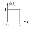
For the Haar case, the mother scaling function is defined by Equation and Figure 4.11.
()
Figure 4.11.
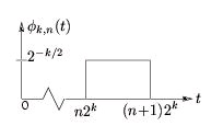
From the mother scaling function, we define a family of shifted and stretched scaling functions
{ φ k , n ( t)} according to Equation and Figure 4.12
()
Figure 4.12.
which are illustrated in Figure 4.13 for various k and n. Equation makes clear the principle that incrementing n by one shifts the pulse one place to the right. Observe from Figure 4.13 that is orthonormal for each k ( i.e. , along each row of figures).
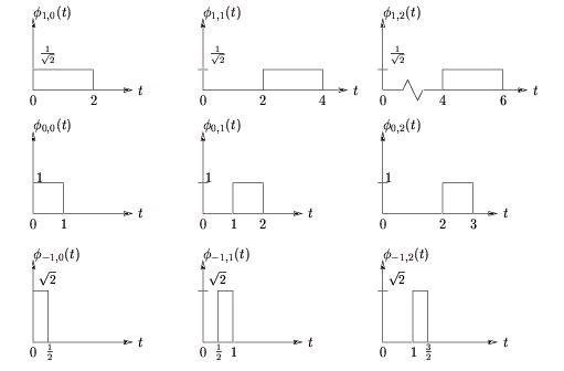


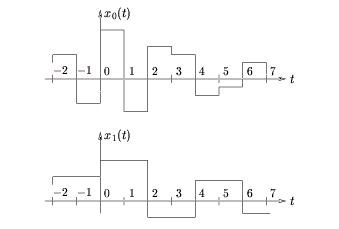
Figure 4.13.
A Hierarchy of Detail in the Haar System*
Given a mother scaling function φ( t)∈ ℒ 2 — the choice of which will be discussed later — let us
construct scaling functions at "coarseness-level-k" and "shift- n" as follows:
Let
us then use Vk to denote the subspace defined by linear combinations of scaling functions at the
k th level:
In the Haar system, for example, V 0 and V 1 consist of signals with
the characteristics of x 0( t) and x 1( t) illustrated in Figure 4.14.
Figure 4.14.
We will be careful to choose a scaling function φ( t) which ensures that the following nesting
property is satisfied: …⊂ V 2⊂ V 1⊂ V 0⊂ V-1⊂ V-2⊂ … coarse detailed In other words, any signal in Vk can be constructed as a linear combination of more detailed signals in V k − 1 . (The Haar
system gives proof that at least one such φ( t) exists.)
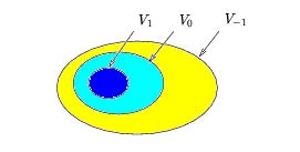


The nesting property can be depicted using the set-theoretic diagram, Figure 4.15, where V − 1 is represented by the contents of the largest egg (which includes the smaller two eggs), V 0 is
represented by the contents of the medium-sized egg (which includes the smallest egg),