DSPA by Douglas Jones, Don Johnson, et al - HTML preview
Download the book in PDF, ePub for a complete version.
Using Euler's relation, we can express the magnitude and phase of this spectrum.
(1.34)
(1.35)
No matter what value of a we choose, the above formulae clearly demonstrate the periodic
nature of the spectra of discrete-time signals. Figure 1.5 shows indeed that the spectrum is a
periodic function. We need only consider the spectrum between
and to unambiguously
define it. When a>0 , we have a lowpass spectrum—the spectrum diminishes as frequency
increases from 0 to —with increasing a leading to a greater low frequency content; for a<0 ,
we have a highpass spectrum (Figure 1.6).
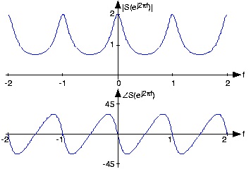
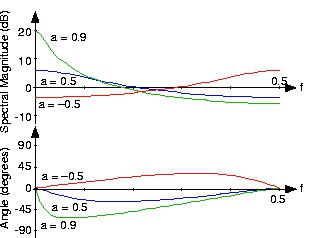


Figure 1.5. Spectrum of exponential signal
The spectrum of the exponential signal ( a=0.5) is shown over the frequency range [-2, 2], clearly demonstrating the periodicity of all discrete-time spectra. The angle has units of degrees.
Figure 1.6. Spectra of exponential signals
The spectra of several exponential signals are shown. What is the apparent relationship between the spectra for a=0.5 and a=–0.5?
Example 1.4.
Analogous to the analog pulse signal, let's find the spectrum of the length- N pulse sequence.
(1.36)
The Fourier transform of this sequence has the form of a truncated geometric series.
(1.37)
For the so-called finite geometric series, we know that
()
for all values of α.


Derive this formula for the finite geometric series sum. The "trick" is to consider the difference
between the series' sum and the sum of the series multiplied by α.
which, after manipulation, yields the geometric sum formula.
Applying this result yields (Figure 1.7.)
()
The ratio of sine functions has the generic form of
, which is known as the discrete-time
sinc function dsinc( x) . Thus, our transform can be concisely expressed as
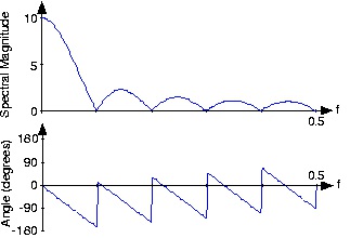
S( ⅇⅈ 2 πf)= ⅇ–( ⅈπf( N−1))dsinc( πf) . The discrete-time pulse's spectrum contains many ripples, the number of which increase with N, the pulse's duration.
Figure 1.7. Spectrum of length-ten pulse
The spectrum of a length-ten pulse is shown. Can you explain the rather complicated appearance of the phase?
The inverse discrete-time Fourier transform is easily derived from the following relationship:
()
Therefore, we find that


()
The Fourier transform pairs in discrete-time are
()
The properties of the discrete-time Fourier transform mirror those of the analog Fourier
transform. The DTFT properties table shows similarities and differences. One important common property is Parseval's Theorem.
()
To show this important property, we simply substitute the Fourier transform expression into the
frequency-domain expression for power.
()
Using the orthogonality relation, the integral equals δ( m− n) , where δ( n) is the unit sample.
Thus, the double sum collapses into a single sum because nonzero values occur only when n= m,
giving Parseval's Theorem as a result. We term
the energy in the discrete-time signal
s( n) in spite of the fact that discrete-time signals don't consume (or produce for that matter)
energy. This terminology is a carry-over from the analog world.
Suppose we obtained our discrete-time signal from values of the product s( t) p Ts ( t) , where the duration of the component pulses in p Ts ( t) is Δ. How is the discrete-time signal energy related to the total energy contained in s( t) ? Assume the signal is bandlimited and that the sampling rate
was chosen appropriate to the Sampling Theorem's conditions.


If the sampling frequency exceeds the Nyquist frequency, the spectrum of the samples equals the
analog spectrum, but over the normalized analog frequency fT . Thus, the energy in the sampled
signal equals the original signal's energy multiplied by T.
1.7. DFT as a Matrix Operation*
Matrix Review
Recall:
Vectors in ℝ N :
Vectors in ℂ N :
Transposition:
1. transpose:
2. conjugate:
1. real:
2. complex:
Matrix Multiplication:
Matrix Transposition:
Matrix transposition involved simply
swapping the rows with columns.
The above equation is Hermitian transpose.
[AT] kn=A nk


Representing DFT as Matrix Operation
Now let's represent the DFT in vector-matrix notation.
Here x is the
vector of time samples and X is the vector of DFT coefficients. How are x and X related:
where
so X= Wx where X is the DFT vector, W is the matrix
and x the time domain vector.
IDFT:
where
is the matrix Hermitian transpose. So,
where x is the time vector,
is the inverse DFT matrix, and X is the DFT vector.
1.8. Sampling theory
Introduction*
Contents of Sampling chapter
Introduction(Current module)
Why sample?


This section introduces sampling. Sampling is the necessary fundament for all digital signal
processing and communication. Sampling can be defined as the process of measuring an analog
signal at distinct points.
Digital representation of analog signals offers advantages in terms of
robustness towards noise, meaning we can send more bits/s
use of flexible processing equipment, in particular the computer
more reliable processing equipment
easier to adapt complex algorithms
Claude E. Shannon
Figure 1.8.
Claude Elwood Shannon (1916-2001)
Claude Shannon has been called the father of information theory, mainly due to his landmark papers on the "Mathematical theory of communication" . Harry Nyquist was the first to state the sampling theorem in 1928, but it was not proven until Shannon proved it 21 years later in the
paper "Communications in the presence of noise" .
Notation
In this chapter we will be using the following notation
Original analog signal x( t)
Sampling frequency Fs
Sampling interval Ts (Note that:
)
Sampled signal xs( n) . (Note that xs( n)= x( nTs) )
Real angular frequency Ω
Digital angular frequency ω. (Note that: ω= ΩTs )
The Sampling Theorem
The Sampling theorem
When sampling an analog signal the sampling frequency must be greater than twice the
highest frequency component of the analog signal to be able to reconstruct the original signal
from the sampled version.
Finished? Have at look at: Proof; Illustrations; Matlab Example; Aliasing applet; Hold
operation; System view; Exercises
Proof*
Sampling theorem
In order to recover the signal x( t) from it's samples exactly, it is necessary to sample x( t) at a rate greater than twice it's highest frequency component.
Introduction
As mentioned earlier, sampling is the necessary fundament when we want to apply digital signal processing on analog signals.
Here we present the proof of the sampling theorem. The proof is divided in two. First we find an
expression for the spectrum of the signal resulting from sampling the original signal x( t). Next we
show that the signal x( t) can be recovered from the samples. Often it is easier using the frequency
domain when carrying out a proof, and this is also the case here.
Key points in the proof
We find an equation for the spectrum of the sampled signal
We find a simple method to reconstruct the original signal
The sampled signal has a periodic spectrum...


The sampled signal has a periodic spectrum...
...and the period is 2π Fs
Proof part 1 - Spectral considerations
By sampling x( t) every Ts second we obtain xs( n). The inverse fourier transform of this time
()
For convenience we express the equation in terms of the real angular frequency Ω using ω= ΩTs .
We then obtain
()
The inverse fourier transform of a continuous signal is
()
From this equation we find an expression for x ( nTs)
()
To account for the difference in region of integration we split the integration in Equation into
subintervals of length
and then take the sum over the resulting integrals to obtain the complete
area.
()
Then we change the integration variable, setting
()
We obtain the final form by observing that ⅇⅈ 2π kn= 1 , reinserting η= Ω and multiplying by


()
To make xs( n)= x( nTs) for all values of n, the integrands in Equation and Equation have to agreee, that is
()
This is a central result. We see that the digital spectrum consists of a sum of shifted versions of
the original, analog spectrum. Observe the periodicity!
We can also express this relation in terms of the digital angular frequency ω= ΩTs
()
This concludes the first part of the proof. Now we want to find a reconstruction formula, so that
we can recover x( t) from xs( n).
Proof part II - Signal reconstruction
For a bandlimited signal the inverse fourier transform is
()
In the interval we are integrating we have:
. Substituting this relation into Equation
we get
()
Using the DTFT relation for Xs( ⅇⅈΩTs) we have
()
Interchanging integration and summation (under the assumption of convergence) leads to


()
Finally we perform the integration and arrive at the important reconstruction formula
()
(Thanks to R.Loos for pointing out an error in the proof.)
Summary
Spectrum sampled signal
Reconstruction formula
Go to Introduction; Illustrations; Matlab Example; Hold operation; Aliasing applet; System
Illustrations*
In this module we illustrate the processes involved in sampling and reconstruction. To see how all
these processes work together as a whole, take a look at the system view. In Sampling and
reconstruction with Matlab we provide a Matlab script for download. The matlab script shows the process of sampling and reconstruction live.
Basic examples
Example 1.5.
To sample an analog signal with 3000 Hz as the highest frequency component requires
sampling at 6000 Hz or above.
Example 1.6.
The sampling theorem can also be applied in two dimensions, i.e. for image analysis. A 2D
sampling theorem has a simple physical interpretation in image analysis: Choose the sampling
interval such that it is less than or equal to half of the smallest interesting detail in the image.
The process of sampling
We start off with an analog signal. This can for example be the sound coming from your stereo at
home or your friend talking.
The signal is then sampled uniformly. Uniform sampling implies that we sample every Ts seconds.
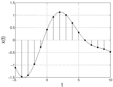
In Figure 1.9 we see an analog signal. The analog signal has been sampled at times t= nTs .
Figure 1.9.
Analog signal, samples are marked with dots.
In signal processing it is often more convenient and easier to work in the frequency domain. So
let's look at at the signal in frequency domain, Figure 1.10. For illustration purposes we take the
frequency content of the signal as a triangle. (If you Fourier transform the signal in Figure 1.9 you will not get such a nice triangle.)
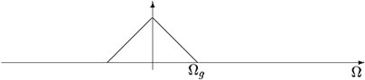


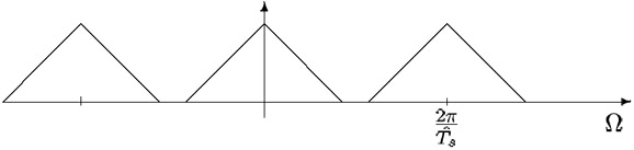
Figure 1.10.
The spectrum X( ⅈΩ) .
Notice that the signal in Figure 1.10 is bandlimited. We can see that the signal is bandlimited
because X( ⅈΩ) is zero outside the interval [– Ωg, Ωg] . Equivalentely we can state that the signal has no angular frequencies above Ωg, corresponding to no frequencies above
.
Now let's take a look at the sampled signal in the frequency domain. While proving the sampling theorem we found the the spectrum of the sampled signal consists of a sum of shifted versions of
the analog spectrum. Mathematically this is described by the following equation:
()
Sampling fast enough
In Figure 1.11 we show the result of sampling