Numerical Methods in Quantum Mechanics by Paolo Giannozzi - HTML preview
Download the book in PDF, ePub, Kindle for a complete version.
+
r2 (E − V (r)) −
+
y(x) = 0
(2.35)
dx2
¯
h2
2
where V (r) = −Zq2e/r for the Coulomb potential. This equation no longer
presents any singularity for r = 0, is in the form of Eq.(1.21), with 2m
2
e
1
g(x) =
r(x)2 (E − V (r(x))) −
+
(2.36)
¯
h2
2
and can be directly solved using the numerical integration formulae Eqs.(1.31)
and Eq.(1.32) and an algorithm very similar to the one of Sect.1.3.2.
Subroutine do mesh defines at the beginning and once for all the values of
√
r,
r, r2 for each grid point. The potential is also calculated once and for all
in init pot. The grid is calculated starting from a minimum value x = −8,
corresponding to Zrmin
3.4 × 10⁻³ Bohr radii. Note that the grid in r does
not include r = 0: this would correspond to x = −∞. The known analytical
behavior for r → 0 and r → ∞ are used to start the outward and inward
recurrences, respectively.
2.3.2
Improving convergence with perturbation theory
A few words are in order to explain this section of the code:
i = icl
ycusp = (y(i-1)*f(i-1)+f(i+1)*y(i+1)+10.d0*f(i)*y(i)) / 12.d0
dfcusp = f(i)*(y(i)/ycusp - 1.d0)
! eigenvalue update using perturbation theory
de = dfcusp/ddx12 * ycusp*ycusp * dx
22
whose goal is to give an estimate, to first order in perturbation theory, of the
difference δe between the current estimate of the eigenvalue and its final value.
Reminder: icl is the index corresponding to the classical inversion point.
Integration is made with forward recursion up to this index, with backward
recursion down to this index. icl is thus the index of the matching point
between the two functions. The function at the right is rescaled so that the
total function is continuous, but the first derivative dy/dx will be in general
discontinuous, unless we have reached a good eigenvalue.
In the section of the code shown above, y(icl) is the value given by Nu-
merov’s method using either icl-1 or icl+1 as central point; ycusp is the value
predicted by the Numerov’s method using icl as central point. The problem
is that ycusp=y(icl).
What about if our function is the exact solution, but for a different problem?
It is easy to find what the different problem could be: one in which a delta func-
tion, v0δ(x−xc), is superimposed at xc ≡x(icl) to the potential. The presence
of a delta function causes a discontinuity (a ”cusp”) in the first derivative, as
can be demonstrated by a limit procedure, and the size of the discontinuity is
related to the coefficient of the delta function. Once the latter is known, we
can give an estimate, based on perturbation theory, of the difference between
the current eigenvalue (for the ”different” potential) and the eigenvalue for the
”true” potential.
One may wonder how to deal with a delta function in numerical integration.
In practice, we assume the delta to have a value only in the interval ∆x centered
on y(icl). The algorithm used to estimate its value is quite sophisticated. Let
us look again at Numerov’s formula (1.32): note that the formula actually provides only the product y(icl)f(icl). From this we usually extract y(icl)
since f(icl) is assumed to be known. Now we suppose that f(icl) has a
different and unknown value fcusp, such that our function satisfies Numerov’s
formula also in point icl. The following must hold:
fcusp*ycusp = f(icl)*y(icl)
since this product is provided by Numerov’s method (by integrating from icl-1
to icl+1), and ycusp is that value that the function y must have in order to
satisfy Numerov’s formula also in icl. As a consequence, the value of dfcusp
calculated by the program is just fcusp-f(icl), or δf .
The next step is to calculate the variation δV of the potential V (r) appearing
in Eq.(2.35) corresponding to δf . By differentiating Eq.(2.36) one finds δg(x) =
−(2me/¯h2)r2δV . Since f (x) = 1 + g(x)(∆x)2/12, we have δg = 12/(∆x)2δf ,
and thus
¯
h2 1
12
δV = −
δf.
(2.37)
2me r2 (∆x)2
First-order perturbation theory gives then the corresponding variation of the
eigenvalue:
δe = ψ|δV |ψ =
|y(x)|2r(x)2δV dx.
(2.38)
23
Note that the change of integration variable from dr to dx adds a factor r to
the integral:
∞
∞
dr(x)
∞
f (r)dr =
f (r(x))
dx =
f (r(x))r(x)dx.
(2.39)
0
−∞
dx
−∞
We write the above integral as a finite sum over grid points, with a single
non-zero contribution coming from the region of width ∆x centered at point
xc =x(icl). Finally:
¯
h2
12
δe = |y(xc)|2r(xc)2δV ∆x = −
|y(xc)|2∆xδf
(2.40)
2me (∆x)2
is the difference between the eigenvalue of the current potential (i.e. with a
superimposed Delta function) and that of the true potential. This expression
is used by the code to calculate the correction de to the eigenvalue. Since in
the first step this estimate may have large errors, the line
e = max(min(e+de,eup),elw)
prevents the usage of a new energy estimate outside the bounds [elw,eip]. As
the code proceeds towards convergence, the estimate becomes better and better
and convergence is very fast in the final steps.
2.3.3
Laboratory
• Examine solutions as a function of n and ; verify the presence of acci-
dental degeneracy.
• Examine solutions as a function of the nuclear charge Z.
• Compare the numerical solution with the exact solution, Eq.(2.29), for the 1s case (or other cases if you know the analytic solution).
• Slightly modify the potential as defined in subroutine init pot, verify
that the accidental degeneracy disappears. Some suggestions: V (r) =
−Zq2e/r1+δ where δ is a small, positive or negative, number; or add an
exponential damping (Yukawa) V (r) = −Zq2e exp(−Qr)/r where Q is a
number of the order of 0.05 a.u..
• Calculate the expectation values of r and of 1/r, compare them with the
known analytical results.
Possible code modifications and extensions:
• Consider a different mapping: r(x) = r0(exp(x) − 1), that unlike the one
we have considered, includes r = 0. Which changes must be done in order
to adapt the code to this mapping?
24
Chapter 3
Scattering from a potential
Until now we have considered the discrete energy levels of simple, one-electron
Hamiltonians, corresponding to bound, localized states. Unbound, delocalized
states exist as well for any physical potential (with the exception of idealized
models like the harmonic potential) at sufficiently high energies. These states
are relevant in the description of elastic scattering from a potential, i.e. pro-
cesses of diffusion of an incoming particle. Scattering is a really important
subject in physics, since what many experiments measure is how a particle is
deflected by another. The comparison of measurements with calculated results
makes it possible to understand the form of the interaction potential between
the particles. In the following a very short reminder of scattering theory is
provided; then an application to a real problem (scattering of H atoms by rare
gas atoms) is presented. This chapter is inspired to Ch.2 (pp.14-29) of the book
of Thijssen.
3.1
Short reminder of the theory of scattering
The elastic scattering of a particle by another is first mapped onto the equivalent
problem of elastic scattering from a fixed center, using the same coordinate
change as described in the Appendix. In the typical geometry, a free particle,
described as a plane wave with wave vector along the z axis, is incident on the
center and is scattered as a spherical wave at large values of r (distance from the
center). A typical measured quantity is the differential cross section dσ(Ω)/dΩ,
i.e. the probability that in the unit of time a particle crosses the surface in the
surface element dS = r2dΩ (where Ω is the solid angle, dΩ = sin θdθdφ, where
θ is the polar angle and φ the azimuthal angle). Another useful quantity is the
total cross section σtot = (dσ(Ω)/dΩ)dΩ. For a central potential, the system
is symmetric around the z axis and thus the differential cross section does not
depend upon φ. The cross section depends upon the energy of the incident
particle.
Let us consider a solution having the form:
f (θ)
ψ(r) = eik·r +
eikr
(3.1)
r
25
with k = (0, 0, k), parallel to the z axis. This solution represents an incident
plane wave plus a diffused spherical wave. It can be shown that the cross section
is related to the scattering amplitude f (θ):
dσ(Ω) dΩ = |f(θ)|2dΩ = |f(θ)|2 sin θdθdφ.
(3.2)
dΩ
Let us look for solutions of the form (3.1). The wave function is in general given by the following expression:
∞
l
χl(r)
ψ(r) =
Alm
Ylm(θ, φ),
(3.3)
r
l=0 m=−l
which in our case, given the symmetry of the problem, can be simplified as
∞
χl(r)
ψ(r) =
Al
Pl(cos θ).
(3.4)
r
l=0
The functions χl(r) are solutions for (positive) energy E = ¯
h2k2/2m with an-
gular momentum l of the radial Schrödinger equation:
¯
h2 d2χl(r)
¯
h2l(l + 1)
+ E − V (r) −
χl(r) = 0.
(3.5)
2m
dr2
2mr2
It can be shown that the asymptotic behavior at large r of χl(r) is
χl(r)
kr [jl(kr) cos δl − nl(kr) sin δl]
(3.6)
where the jl and nl functions are the well-known spherical Bessel functions,
respectively regular and divergent at the origin. These are the solutions of the
radial equation for Rl(r) = χl(r)/r in absence of the potential. The quantities
δl are known as phase shifts. We then look for coefficients of Eq.(3.4) that yield the desired asymptotic behavior (3.1). It can be demonstrated that the cross section can be written in terms of the phase shifts. In particular, the differential
cross section can be written as
2
dσ
1
∞
=
(2l + 1)eiδl sin δlPl(cos θ) ,
(3.7)
dΩ
k2 l=0
while the total cross section is given by
4π ∞
2mE
σtot =
(2l + 1) sin2 δl
k =
.
(3.8)
k2
¯
h2
l=0
Note that the phase shifts depend upon the energy. The phase shifts thus con-
tain all the information needed to know the scattering properties of a potential.
26
3.2
Scattering of H atoms from rare gases
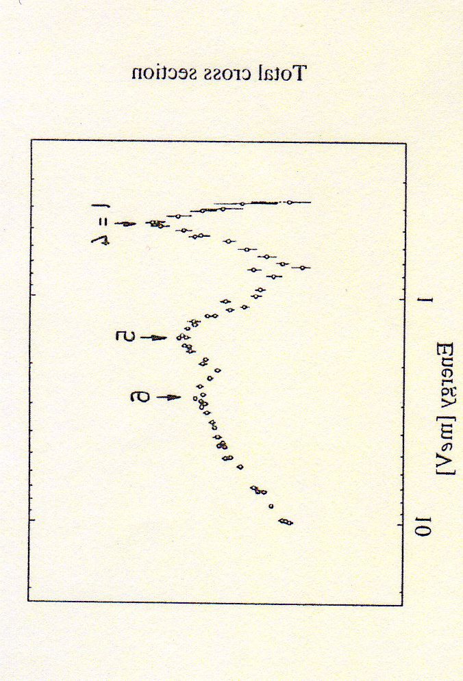
The total cross section σtot(E) for the scattering
of H atoms by rare gas atoms was measured by
Toennies et al., J. Chem. Phys. 71, 614 (1979).
At the right, the cross section for the H-Kr sys-
tem as a function of the energy of the center of
mass. One can notice “spikes” in the cross sec-
tion, known as “resonances”. One can connect
the different resonances to specific values of the
angular momentum l.
The H-Kr interaction potential can be modelled quite accurately as a Lennard-
Jones (LJ) potential:
σ 12
σ 6
V (r) =
− 2
(3.9)
r
r
where
= 5.9meV, σ = 3.57˚
A. The LJ potential is much used in molecular and
solid-state physics to model interatomic interaction forces. The attractive r−6
term describes weak van der Waals (or “dispersive”, in chemical parlance) forces
due to (dipole-induced dipole) interactions. The repulsive r−12 term models the
repulsion between closed shells. While usually dominated by direct electrostatic
interactions, the ubiquitous van der Waals forces are the dominant term for the
interactions between closed-shell atoms and molecules. These play an important
role in molecular crystals and in macro-molecules. The LJ potential is the first
realistic interatomic potential for which a molecular-dynamics simulation was
performed (Rahman, 1965, liquid Ar).
It is straightforward to find that the LJ potential as written in (3.9) has a minimum Vmin = − for r = σ, is zero for r = σ/21/6 = 0.89σ and becomes
strongly positive (i.e. repulsive) at small r.
3.2.1
Derivation of Van der Waals interaction
The Van der Waals attractive interaction can be described in semiclassical terms
as a dipole-induced dipole interaction, where the dipole is produced by a charge
fluctuation. A more quantitative and satisfying description requires a quantum-
mechanical approach. Let us consider the simplest case: two nuclei, located
in RA and RB, and two electrons described by coordinates r1 and r2. The
Hamiltonian for the system can be written as
¯
h2
q2
¯
h2
q2
H
=
−
∇2 −
e
−
∇2 −
e
(3.10)
2m
1
|r
2
1 − RA|
2m
|r2 − RB|
q2
q2
q2
q2
−
e
−
e
+
e
+
e
,
|r1 − RB|
|r2 − RA|
|r1 − r2|
|RA − RB|
where ∇i indicates derivation with respect to variable ri, i = 1, 2. Even this
“simple” hamiltonian is a really complex object, whose general solution will be
the subject of several chapters of these notes. We shall however concentrate on
27
the limit case of two Hydrogen atoms at a large distance R, with R = RA −RB.
Let us introduce the variables x1 = r1−RA, x2 = r2−RB. In terms of these new
variables, we have H = HA + HB + ∆H(R), where HA (HB) is the Hamiltonian
for a Hydrogen atom located in RA (RB), and ∆H has the role of “perturbing
potential”:
q2
q2
q2
q2
∆H = −
e
−
e
+
e
+ e .
(3.11)
|x1 + R|
|x2 − R|
|x1 − x2 + R|
R
Let us expand the perturbation in powers of 1/R. The following expansion,
valid for R → ∞, is useful:
1
1
R · x
3(R · x)2 − x2R2
−
+
.
(3.12)
|x + R|
R
R3
R5
Using such expansion, it can be shown that the lowest nonzero term is
2q2
(R · x1)(R · x2)
∆H
e
x1 · x2 − 3
.
(3.13)
R3
R2
The problem can now be solved using perturbation theory. The unperturbed
ground-state wavefunction can be written as a product of 1s states centered
around each nucleus: Φ0(x1, x2) = ψ1s(x1)ψ1s(x2) (it should actually be anti-
symmetrized but in the limit of large separation it makes no difference.). It is
straightforward to show that the first-order correction, ∆(1)E = Φ0|∆H|Φ0 ,
to the energy, vanishes because the ground state is even with respect to both x1
and x2. The first nonzero contribution to the energy comes thus from second-
order perturbation theory:
| Φi|∆H|Φ0 |2
∆(2)E = −
(3.14)
E
i>0
i − E0
where Φi are excited states and Ei the corresponding energies for the unper-
turbed system. Since ∆H ∝ R−3, it follows that ∆(2)E = −C6/R6, the well-
known behavior of the Van der Waals interaction.1 The value of the so-called C6 coefficient can be shown, by inspection of Eq.(3.14), to be related to the product of the polarizabilities of the two atoms.
3.3
Code: crossection
Code crossection.f902, or crossection.c3, calculates the total cross section σtot(E) and its decomposition into contributions for the various values of the
angular momentum for a scattering problem as the one described before.
The code is composed of different parts. It is always a good habit to verify
separately the correct behavior of each piece before assembling them into the
final code (this is how professional software is tested, by the way). The various
parts are:
1Note however that at very large distances a correct electrodynamical treatment yields a
different behavior: ∆E ∝ −R−7.
2http://www.fisica.uniud.it/%7Egiannozz/Corsi/MQ/Software/F90/crossection.f90
3http://www.fisica.uniud.it/%7Egiannozz/Corsi/MQ/Software/C/crossection.c
28
1. Solution of the radial Schrödinger equation, Eq.(3.5), with the Lennard-Jones potential (3.9) for scattering states (i.e. with positive energy). One can simply use Numerov’s method with a uniform grid and outwards
integration only (there is no danger of numerical instabilities, since the
solution is oscillating). One has however to be careful and to avoid the
divergence (as ∼ r−12) for r → 0. A simple way to avoid running into
trouble is to start the integration not from rmin = 0 but from a small but
nonzero value. A suitable value might be rmin ∼ 0.5σ, where the wave
function is very small but not too close to zero. The first two points can be
calculated in the following way, by assuming the asymptotic (vanishing)
form for r → 0:
2m σ12
2m σ12
χ (r)
χ(r)
=⇒
χ(r)
exp
−
r−5
(3.15)
¯
h2 r12
25¯
h2
(note that this procedure is not very accurate because it introduces and
error of lower order, i.e. worse, than that of the Numerov’s algorithm.
In fact by assuming such form for the first two steps of the recursion,
we use a solution that is neither analytically exact, nor consistent with
Numerov’s algorithm).
The choice of the units in this code is (once again) different from that of
the previous codes. It is convenient to choose units in which ¯
h2/2m is a
number of the order of 1. Two possible choices are meV/˚
A2, or meV/σ2.
This code uses the former choice. Note that m here is not the electron
mass! it is the reduced mass of the H-Kr system. As a first approximation,
m is here the mass of H.
2. Calculation of the phase shifts δl(E). Phase shifts can be calculated by
comparing the calculated wave functions with the asymptotic solution at
two different values r1 and r2, both larger than the distance rmax beyond
which the potential can be considered to be negligible. Let us write
χl(r1) = Akr1 [jl(kr1) cos δl − nl(kr1) sin δl]
(3.16)
χl(r2) = Akr2 [jl(kr2) cos δl − nl(kr2) sin δl] ,
(3.17)
from which, by dividing the two relations, we obtain an auxiliary quantity
K
r2χl(r1)
jl(kr1) − nl(kr1) tan δl
K ≡
=
(3.18)
r1χl(r2)
jl(kr2) − nl(kr2) tan δl
from which we can deduce the phase shift:
Kjl(kr2) − jl(kr1)
tan δl =
.
(3.19)
Knl(kr2) − nl(kr1)
The choice of r1 and r2 is not very critical. A good choice for r1 is about
at rmax. Since the LJ potential decays quite quickly, a good choice is
r1 = rmax = 5σ. For r2, the choice is r2 = r1 + λ/2, where λ = 1/k is the
wave length of the scattered wave function.
29
3. Calculation of the spherical Bessel functions jl and nl. The analytical
forms of these functions are known, but they become quickly unwieldy for
high l. One can use recurrence relation. In the code the following simple
recurrence is used:
2l + 1
zl+1(x) =
zl(x) − zl−1(x),
z = j, n
(3.20)
x
with the initial conditions
cos x
sin x
sin x
cos x
j−1(x) =
,
j0(x) =
;
n−1(x) =
,
n0(x) = −
.
x
x
x
x
(3.21)
Note that this recurrence is unstable for large values of l: in addition to
the good solution, it has a ”bad” divergent solution. This is not a serious
problem in practice: the above recurrence should be sufficiently stable up
to at least l = 20 or so, but you may want to verify this.
4. Sum the phase shifts as in Eq.(3.8) to obtain the total cross section and a graph of it as a function of the incident energy. The relevant range of
energies is of the order of a few meV, something like 0.1 ≤ E ≤ 3 ÷ 4
meV. If you go too close to E = 0, you will run into numerical difficulties
(the wave length of the wave function diverges). The angular momentum
ranges from 0 to a value of lmax to be determined.
The code writes a file containing the total cross section and each angular mo-
mentum contribution as a function of the energy (beware: up to lmax = 13; for
larger l lines will be wrapped).
3.3.1
Laboratory
• Verify the effect of all the parameters of the calculation: grid step for in-
tegration, rmin, r1 = rmax, r2, lmax. In particular the latter is important:
you should start to find good results when lmax ≥ 6.
• Print, for some selecvted values of the energy, the wave function and its
asymptotic behavior. You should verify that they match beyond rmax.