R Programming in Statistics by Balasubramanian Thiagarajan - HTML preview
Download the book in PDF, ePub, Kindle for a complete version.
Introduction 7
Unique features of R programming: 10
Instal ation R base software:
10
Instal ation of RStudio: 18
Why a programming language like R should be learnt by a non-programmer? 23
RStudio ideal settings & RGui 24
Updating R and RStudio: 28
RGui: (R Base software) 31
Print: 36
GUI Preferences: 39
View menu: 40
Packages menu: 43
Windows Menu : 48
Help Menu: 50
Getting started: 54
R-Studio 54
Console: 56
Types of Data in R 79
Data An Introduction 79
Operators in R Programming 140
Assignment Operators: 164
These operators are used to assign values to vectors.
164
Left assignment: 164
<- 164
= 164
<<- 164
These operators can be used interchangeably. 164
c indicates concatenate in R language. 164
Miscel aneous operators: 167
R Programming in Statistics
Statistical summary function: 169
Simulation and statistical distributions:
171
Functions in R Programming 177
List function:
203
Data Entry in R Programming
233
Data Analysis in R Programming 255
Exploratory data analysis: 263
Measures of central tendency: 267
One Sample T-Testing: 283
Hypothesis Testing in R Programming 283
Two Sample T-Testing: 285
Directional Hypothesis: 287
One Sample Mu test:
288
Bootstrapping in R Programming:
291
Time series analysis using R: 294
Tidyverse 299
Anova 320
Post-hoc tests in R: 333
Descriptive Statistics
335
Mean: 341
Median: 343
Interquartile range:
344
Standard deviation and variance:
344
Summary: 347
Coefficient of variation: 347
Mode: 347
Correlation: 351
Mosaic plot: 353
Bar plot:
353
Histogram: 355
Prof. Dr Balasubramanian Thiagarajan
5
Dot plot: 357
Scatter plot: 357
Exploratory Data Analysis 359
Regression Analysis using R 364
Pie chart: 373
R Charts and Graphs
373
Bar plot:
377
Boxplots: 382
Line graphs using R:
389
R Scatterplots:
395
Creating the scatterplot: 396
R Programming in Statistics
R is a language and environment for statistical and graphics. This GNU project is similar to the “S” language and environment that was developed by Bell laboratories. Even though R can be considered as a different implementation of S, there are some important differences. Most of the code written for S runs unaltered under R.
In 1992, Ross Ihaka and Robert Gentleman created R at the University of Aukland. This was to enable the students to use this as a statistical tool. Initial version was released in 1995. Currently it is being maintained by the R Development Core Team.
R provides a variety of statistical (linear and non-linear modelling, classical statistical tests, time series analysis, classification, clustering etc). It also provides graphical techniques and is highly extensible.
One major strength of R is the ease with which well-designed publication quality plots can be produced, including mathematical symbols and formulae when needed.
1. It is a free and open source tool.
2. It has a large community of users
3. It is an independent platform and can be run without a compiler.
4. Can be considered to be the Gateway for lucrative career 5. Has a robust visualization library - R comprises libraries like ggplot2, plotly that offer aesthetic graphical plots to its users. R is recognized for its stunning visualizations which gives it an edge over Data science programming languages.
6. Used in almost every Industry
7. Distributed computing - In distributive computing, tasks are spit between multiple processing nodes to reduce processing time and to increase efficiency. R has packages lid ddr and multiDplyr that enable it to use distributed computing to process large data sets.
8. Iterfacing with Databases - R contains several packages that enable it to interact with databases like ROra-cle, Open database connectivity Protocol, Rmy SQL, etc.
9. Data Variety - R can handle a variety of structured as well as unstructured data. It also provides various data modeling and data operation facilities due to its interaction with databases.
10. Compatible with other programming languages - Most of the functions are written in R itself, C, C++
or Fortran can be used for computational y heavy tasks. Java, .NET, Python can also be used to manipulate objects directly.
Prof. Dr Balasub
R Prram
og a
ra nian Thi
mmin aga
g in Stra
at jiasn
tics
7
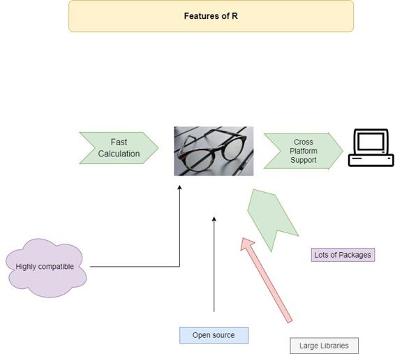
R code can be run without any compiler. It is an interpreted language and hence compiler is not need to run the code. Calculations are done with vectors. R is actual y a vector language, hence anyone can add functions to a single vector without putting in a loop. R is hence powerful and faster than other languages.
Feature of R include:
1. Data inputs and data management. Data inputs such as data type, importing data and keyboard typing.
2. Data management such as data variables, operators.
Pros of R language:
1. It is the most comprehensive statistical analysis package, and new ideas often appear first in R.
2. R is an open source and can be run anywhere any time.
3. It is cross platform and runs on many operating systems.
Cons of R language:
1. The quality of some packages in R is less than perfect.
2. There is no customer support of R language.
The R Environment:
This is an integrated suite of software that can be used for data manipulation, calculation and graphical display. It includes:
1. An effective data handling and storage facility
2. A suite of operators for calculations on arrays, in particular matrices 3. A large, coherent, integrated collection of intermediate tools for data analysis 4. Graphical facilities for data analysis and display either on-screen or on hard copy 5. A well developed, simple and effective programming language which includes conditions, loops, user defined recursive functions and input and output facilities.
The term environment is intended to characterize it as a ful y planned and coherent system rather than an incremental accretion of very specific inflexible tools.
R has been designed around a true computer language, and it allows users to add additional functionality by defining new functions. R also has its own LaTeX like document format which is used to supply comprehensive documentation both on-line in a number of formats and in hard copy.
R Programming in Statistics
Prerequisites before learning R:
Before one jumps into R, it is highly recommended that they possess some basic knowledge of a few topics. These include:
1. Basic understanding of statistics, mathematics, and probability.
2. General understanding of data science and the process involved.
3. Basic understanding of various types of graphs and data representation techniques.
Prof. Dr Balasubramanian Thiagarajan
9
Unique features of R programming:
Since there are a large number of packages are available, there are many handy features in R. They include: 1. Its ability to perform directly on vectors and hence does not require too much looping.
2. It can pull data from APIs, servers, SPSS files and many other formats.
3. It is very useful for web scraping.
4. It can perform multiple complex mathematical operations with a single command.
5. It can create attractive reports combined with plain text with code and visualizations of the results if R
markdown feature is used.
6. Since the user base is large, new ideas and technologies appear in the R community first.
Instal ation R base software:
Step I : R Base needs to be installed first. R is mainatined by an international team of developers and the software is available in multiple languages in their webpage “The Comprehensive R Archive Network”. From here the version appropriate to the User’s operating system can be downloaded. R is available for: Windows operating system
Mac OS
Various flavors of linux
Installing R in windows is fairly simple as it comes bundled with its own installer which takes care of the entire instal ation process. As the user has to do is to double click on the downloaded binary file.
Step II: The windows executable file after being downloaded is double clicked to begin the instal ation process. All the user has got to do is keep clicking the next button till the confirmation screen appears saying that the process of instal ation is over. If the user is using a computer that is shared by others then Install for all users radio button needs to be selected to make the software available to all the users using the system.
The first screen allows the user to choose the language of instal ation. R software is available in various common languages. It is preferable to allow the instal ation into the default folder created by the installer than customizing the process of instal ation. Since the user will have to install an Integrated Development Environment (IDE) software after installing R base software it will be fairly straight forward for the IDE to use R
base software as it has been installed in to the default folder R Programming in Statistics


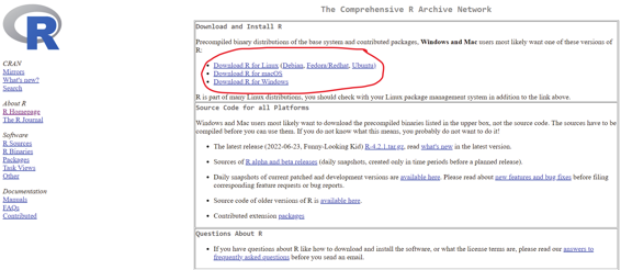


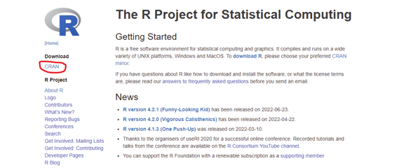

Image showing CRAN webpage where the various flavors of R are available for download Image showing the official R project webpage
Prof. Dr Balasubramanian Thiagarajan
11
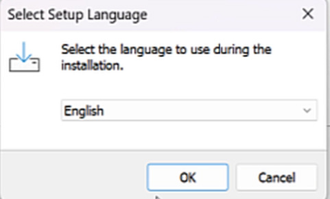


In the first screen shown above the language of the
instal ation needs to be chosen before clicking on
the OK button
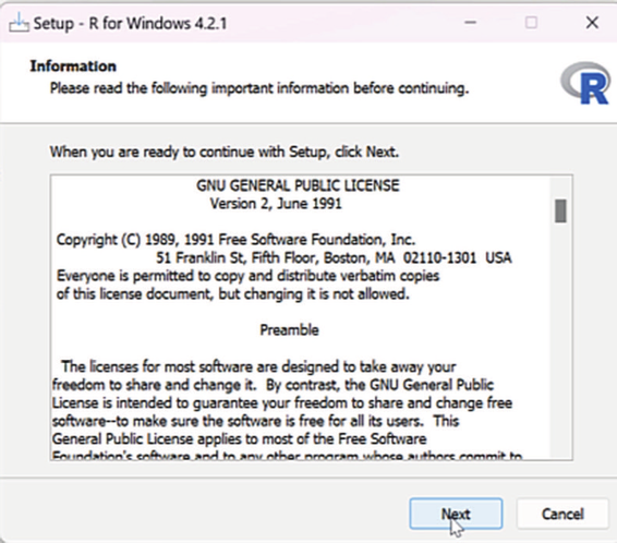
Image showing GNU licence screen which needs to be accepted by clicking the next button
R Programming in Statistics


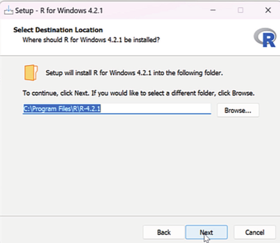

Image showing the screen that gives the choice of destination of location to the user. It is ideal for the user to allow the default settings by clicking on the next button. If the system has an SSD disk installed then instal ation is preferred in that disk as it would speed up the application process. If the user’s system has multiple hard disks and one of them happens to be a SSD it is preferable to install it there.
R comes with both 32 bit AND 64 bit versions. The user will have a dilemma in choosing which version to use. Actual y it does not matter as both versions use 32-bit integers, which indicates that they compute numbers to the same numerical precision. The difference occurs in the way each version manages the system memory. 64-bit R uses 64-bit memory pointers and 32-bit uses 32-bit memory pointers, this means that 64-bit has a larger memory space to use.
It should be pointed out that 32-bit builds of R are slightly faster than 64-bit builds. On the flip side 64-bit builds can handle larger files and data sets with fewer memory management problems. Hence if the operating system does not support 64-bit programs, or the installed RAM is less than 4 GB then it is ideal to install 32-bit R software. If the system supports 64-bit then the installer would install both versions of R.
Prof. Dr Balasubramanian Thiagarajan
13


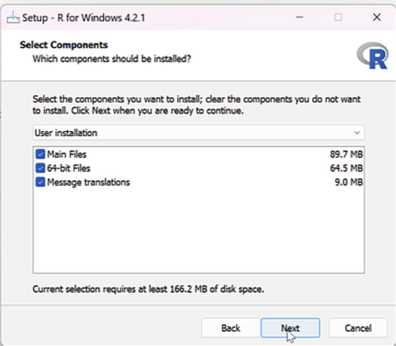


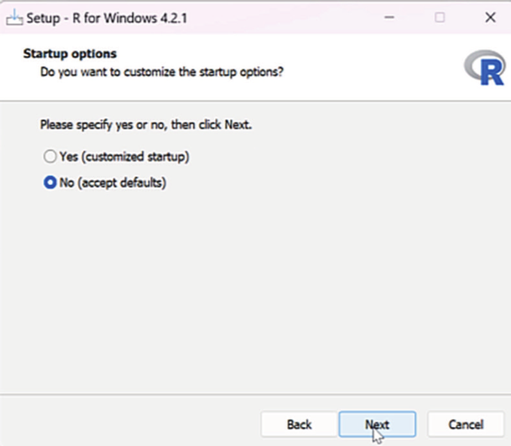

Image showing the screen that prompts user to select the desired components for instal ation. The user should choose the Main Files, 64-bit files if desired and Message translations if needed. The default settings is preferred and advisable. If the user wants 32 bit instal ation only, then 64-bit Files can be unchecked.
Image showing startup options window
R Programming in Statistics


Startup options:
When R is started, it will by default source a .Rprofile file if it exists. This allows the user to automatical y tweak the R settings to meed the everyday needs. The startup package extends the default R startup process by allowing the user to put multiple startup scripts in a common "Rprofile.d" directory. If customization is needed for startup then during instal ation "customize startup radio button is selected" and in the ensuing window the customized file is pointed to enable customized startup. The user can have one file to configure the default CRAN repository and another one to configure their personal devtools settings. The user can also use a "Renviron.d" directory with mulitple files defining different environmental variables like language etc,. One file could contain the private GITHUB_pat key.
This customization is needed for advanced users who are well versed in R language scripting and advanced computing techniques. This step is narrated not to daunt the first time user but to il ustrate the extensive customizations that are available within R environment which can be used if desired.
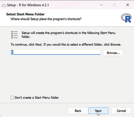
Image showing the prompt screen that allows the user to select the start menu folder where R shortcut is going to be stored. Here if the next button is clicked the defualt folder named R will be created in startup menu folder.
Prof. Dr Balasubramanian Thiagarajan
15


A small tip regarding the choice of instal ation folder in R programing instal ation: If the user desires to install this software in a company owned computer where usual y C drive access is not provided to the user as part of the company policy it is important to change the instal ation drive to where the user has access to. Instal ation will not progress if the user does not have access to the drive where installation folder is being created.
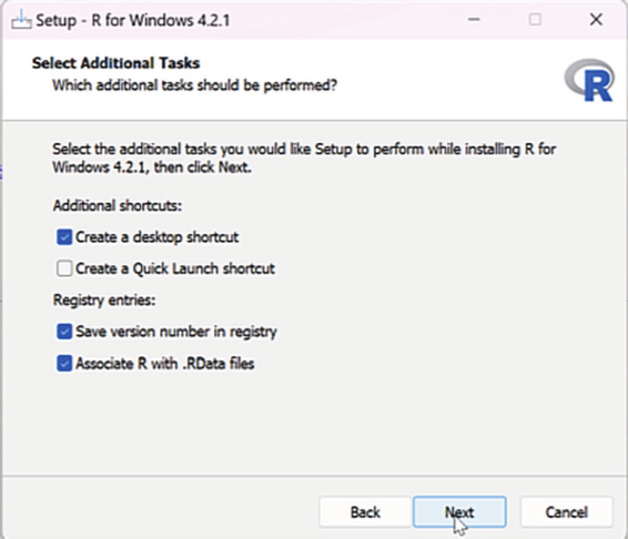
Image showing the instal ation screen where additional tasks can be selected during instal ation process.
In the image shown above the additional tasks that needs to be performed has been selected by default. The additional tasks already selected by default is sufficient for the instal ation to proceed. If the user desires to create a quick launch short cut then that box needs to be checked. Save version number in the registry helps in the process of identification of updates released if any. Another setting that has been chosen by default is Associate R with .RData files. This setting which is chosen by default will ensure that R files are associated with this software.
R Programming in Statistics


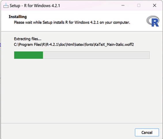

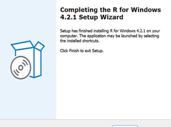
Image showing the file extraction process progressing
Image showing confirmation screen showing instal ation has been compteted successfully
Prof. Dr Balasubramanian Thiagarajan
17


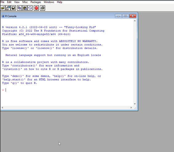

Image showing the R interface
Instal ation of RStudio:
RStudio is one of the most popular IDE (Integrated Development Environment) for working with R programming language. R studio should be installed only after instal ation of R base software. This would serve as a front end of R programming language.
Advantages of RStudio:
There are multiple ways to interface with R. Some common interfaces are the basic R GUI, R Commander and RStudio. Among these front end software for R programming language RStudio happens to be the best.
RStudio is designed to make it easy to write scripts. As soon as a new script is created, the windows within RStudio session adjusts automatical y so that the user would be able to see both the script and the results in the console when the syntax is run. It has also the ability to call up potential syntax options while keying the scripts just by using the tab key.
RStudio makes it convenient to view and interact with the objects stored in the environment.
R Programming in Statistics


RStudio makes it easy to set the working directory and access files on the computer. This is more so true while working on windows environment. Without RStudio setting the working directory is the most tedious process in windows environment. Using RStudio one can navigate to folders on the computer in the “Files”
window, view any files that are available in that folder, and set that folder as the working directory.
RStudio makes graphics much more accessible to a casual user. With the basic R programming one has to go to some lengths to save graphiscs, but with RStudio it has a window that makes the job simple.
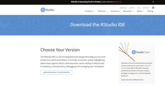
Image showing the web page from which RStudio can be downloaded.
One of the easiest ways to reach this web page is to perform a google search for the term R Studio. It will take the user to the R studio page. In the RStuio web page free version of the software is chosen for the download.
After the download is complete it can be executed for the instal ation process to continue.
Prof. Dr Balasubramanian Thiagarajan
19


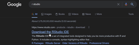


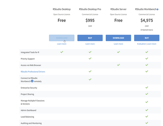

Image showing the google search result for RStudio
Image showing the download page for RStudio. RStudio Desktop Free version is chosen for download R Programming in Statistics


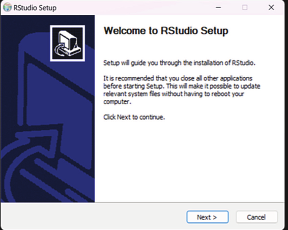


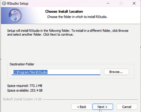

Image showing the RStudio setup screen.
Image shwoing the screen where instal ation location can be chosen Prof. Dr Balasubramanian Thiagarajan
21


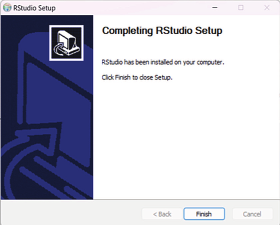


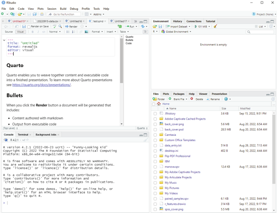

Image showing RStudio setup completed screen
Image showing RStudio window
R Programming in Statistics
Why a programming language like R should be learnt by a non-programmer?
It must be stressed that R is a powerful programming language. It is used for a lot of quantitative data analysis, it has grown over the years to become a real y powerful tool that specializes in handling data and performing customized computations with quantitative and qualitative data.
R language can be used to perform:
Statistical analysis
Corpus analysis
Development of online dashboards
Connection to social media APIs for data collection
Creation of reporting systems to provide individualized feedback to research participants.
Writing research articles, books and blog posts.
Learning new tools to analyze data is always essential. Theories change over time, and new insights into certain social phenomena are published every day. Knowledge might get outdated quite quickly. It should be pointed out that analytical techniques like mean, median, mode, quartiles, standard deviation etc., have remained the same. Programming languages allows the user to look at the data from a different angle.
Prof. Dr Balasubramanian Thiagarajan
23


RStudio ideal settings & RGui
For the first time user it is always better to adjust the following settings so that life for a programmer becomes that much easier. These settings are listed under Tools / Global options. Global options can be invoked by clicking on Tools button and selecting Global options from the drop down menu.
Image showing Global options listed under Tools menu
R Programming in Statistics


The following changes to Global options are recommended:
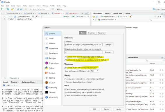
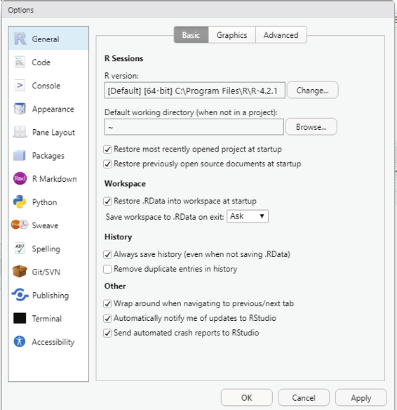
1. In the first tab (General > Basic) one should make one of the most signigicant changes. All options that starts with “Restore” should be deactivated. This will ensure that every time the user starts RStudio, it begins with a clean slate. It would seem counter-intuitive not to restart everything from where the user has left off, but is essential to make all the projects easily reproducible. Disabling this feature would also make it easy for col aborative work. The settings that need to be unchecked include:
. Restore most recently opened project at startup.
. Restore previously open source documents at startup.
. Restore .Rdata into workspace at startup.
Image showing the Basic tab under General options. Note the highlighted settings needs to be unchecked.
RStudio wil l restart to carry out the desired changes.
Prof. Dr Balasubramanian Thiagarajan
25


2. In the same tab under workspace, Never is selected for the setting Save workspace to .RData on exit. One could think that it is wise to keep intermediary results stored form one R session to another. Unchecking this setting would avoid future headaches.
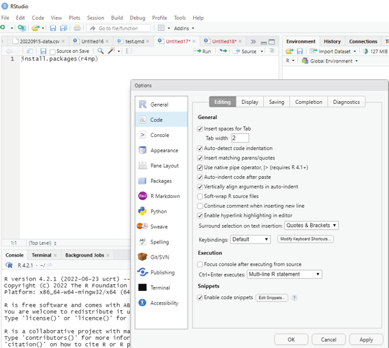
3. In the Code > Editing tab it is made sure that at least the first five options are ticked. Especial y the Au-to-indent code after paste. This setting will save time when the user tries to format the coding appropriately, making it easier to read and comprehend. Indentation is the primary way of making the code look more readable and less like a series of random characters.
Image showing ideal Code settings that are preferred by the author.
At this point it should be stressed that there is no such thing as ideal settings. Settings are nothing but personal preference of the user. The fact that these settings are available ensures certain amount of flexibility to the user to manipulate. Individual users should be encouraged to play around with these settings and settle down with the most comfortable ones for their use. These are nothing but recommendations for the novice user.
R Programming in Statistics


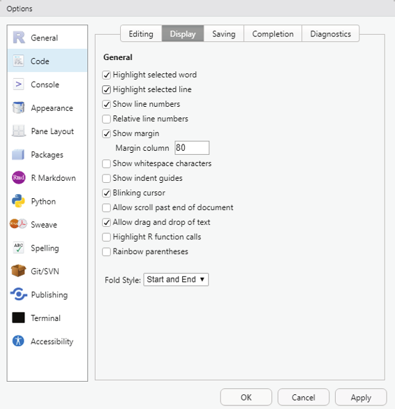

4. In the Display tab under Code menu the first three options should be selected. Among these settings one particular setting is rather useful i.e., Highlight selected line. This is rather helpful in analyzing more complicated code, as it is helpful to see where the cursor is. One can also customize the workspace still further. The visual y most impactful way to alter the default appearance of RStudio is to select Appearance setting and pick a completely different theme. There are no absolulte right and wrongs here. It is purely personal preference of the user.
Image showing ideal Display settings chosen under Code menu Prof. Dr Balasubramanian Thiagarajan
27


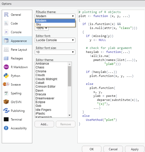

Image showing Appearance setting where RStudio themes can be changed to suit user preference.
Updating R and RStudio:
When software is being updated, one needs to update R and RStudio separately from each other. Even though R and RStudio work closely with each other, they still constitute separate pieces of software. RStudio and R cannot update on their own because some packages may not work after switching to the new version.
If something goes wrong the user can stil l downgrade R version in RStudio. After the new version is installed, the previously installed packages will not go to next version. Extra procedures need to be performed.
Upgrading R on windows could be tricky. Easiest option would be to uninstall R and then install the new version. One needs to reinstall all required packages with the new version of R and then delete the old library once they are not needed.
R Programming in Statistics
Updating R using installr package:
The {installr} package offers a set of R functions for the instal ation and updation of software. This package is available for windows OS only. The following code should be used:
# instal ing/loading the package:
if(!require(instal r)) {
install.packages(“instal r”); require(instal r)} #load / install+load instal r
# using the package:
updateR() # this will start the updating process of your R instal ation. It will check for newer versions, and if one is available, will guide you through the decisions you’d need to make.
Running this fuction will perform the following steps:
1. Check what is the latest R version. If the current installed R version is up-do-date, the function ends (and returns FALSE).
2. If a newer version of R is available, the user would be asked if to review the News of the latest R version in order to decide if to install the newest R or not.
3. If the user wishes to update, the function will download and install the latest R version. The next button needs to be pressed by the user.
4. Once instal ation is done, the user should press “any key” and the function will proceed with copying all of the packages from the old R instal ation into the newer R instal ation.
5. The user can erase all of the packages in the old R instal ation.
6. After the packages are moved (and the old ones probably erased), the user will get the option to update all the packages in the new version of R.
If the user wishes to upgrade R, and only want the packages to be moved and not copied then the following command is used:
# instal ing/loading the package:
if(!require(instal r)) { install.packages(“instal r”); require(instal r)} #load / install+load instal r updateR(F, T, T, F, T, F, T) # install, move, update.package, quit R.
Another way of updating R is to simply download the newest version and run it. It will overwrite the previous version. When R is being updated the biggest challenge is that the personal library of packages dont work anymore. If the user desires to copy the personal library then it can be copied to a new location and ensuring that the new version of R recognizes it. Some users feel that it is a good time to start with a clean slate and only install packages that are needed.
Prof. Dr Balasubramanian Thiagarajan
29


Updating R studio:
RStudio can be updated from within the software. Check for Update link can be found under Help menu. It will ensure that the new version is downloaded and installed over the old version.
Image showing Check for Updates link under Help menu in RStudio.
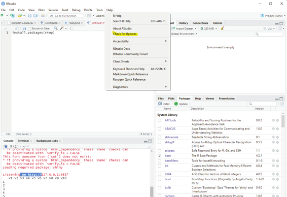
Updating installed packages:
Installed packages can be updated by clicking on Check for Package updates link listed under Tools Menu.
Similarly new packages can be installed by clicking on Install Package menu listed under Tools Menu. RStudio provides an easy way of updating and installing the packages desired by the user.
R Programming in Statistics


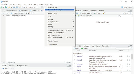

Image showing Package update link under Tools menu in RStudio that can be used to update installed packages.
RGui: (R Base software)
RGui which is the graphic user interface that is installed as part of R instal tion can be used to compile and run R code. It comes with a Console window where codes can be written and run. It is always better to use along with IDE like RStudio in order to make its use rather simple. Use of IDE saves a lot of time for the user.
RGui can also be used for R programming without instal ation of IDE like RStudio. Installing RStudio along with R real y makes the life of the user comfortable. User must be aware of RGui and its features. This will ensure that the user becomes a better R programmer.
Prof. Dr Balasubramanian Thiagarajan
31


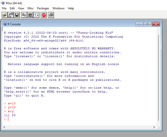

Image showing RGui interface
RGui has the fol woing menu at the top:
File
Edit
View
Misc
Packages
Windows
Help
R Programming in Statistics


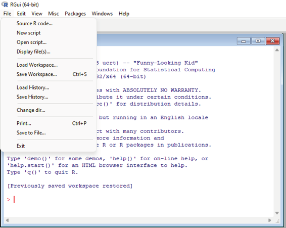

Image showing Top Menu of RGui
Under the file menu there are 12 submenus:
Source R Code - This submenu can be used to load R code file from the folder where it is stored. This can be used to reuse function that has been created in another R script. The source file caues R to accept its input from the named file. The input is read and parsed from that file until the end of the file is reached, then the parsed expressions are evaluated sequential y in the chosen environment.
New script:
To start writing a new R script in R base click on the File menu and then click on New script menu. On clicking the New script menu a R scripting window will open. Scripts can be written / typed in the scripting window and the same would be seen in the R console window.
Prof. Dr Balasubramanian Thiagarajan
33


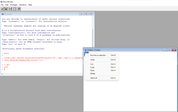

Image showing R editor opening up after the menu New script is selected and clicked.
Any script that is written in R editor will be incorported into the console window. The code lines can be selected and on right clicking the menu as shown above will open. On choosing the code lines and clicking on Run line / selection menu the code will run in the console.
Open script menu:
This can be used to open a saved R script. Programmers usual y save the script that they have created. The saved script can be opened from within R base using open script menu. On clicking Open script menu a file browser window will open from where the user can select the script that needs to be run.
R Programming in Statistics


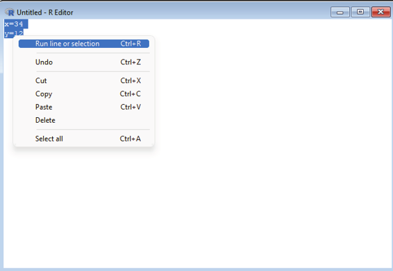

Image showing the code line that needs to be run selected and on right clicking a submenu opens up. On choosing Run line or selection the selected code runs. If undo is selected the typed code can be undone.
Similary cut / copy / paste can be used to cut, copy or paste the code. Delete menu can b e used to delete the code typed. On selecting Select all menu the entire code is selected.
Display files Menu:
On clicking this drop down menu listed under File in R Base window a file browser window will open displaying the contents of my documents folder. This menu can be used to open the file browser window. Default location where R files are stored is My documents and hence this menu opens up this folder on default.
Load workspace:
On clicking this menu file browser window opens up displaying the contents of My documents folder. This is the default location where R language scripts and objects are saved as work space. These saved files can be loaded again into the R programming console by clicking on this submenu. All the objects and functions that are created by the user can be saved in a file with a suffix .RData by using the save() function or the save.
image() function in the command prompt. The assigned file name goes into the bracket.
Exact command - >save(file=”d:/filename.RData”)
>save.image(“d:/filename.RData”) Prof. Dr Balasubramanian Thiagarajan
35


These commands will be discussed in detail in later chapters.
Save workspace:
The user is prompted to save the R script as well as the objects in the console on exiting the software. The save file has a suffix of .R. The default location where the workspace is usual y saved is Documents or My Documents folder as the case may be. The user of course can change the file save location when the file browser window opens up prompting the user to save the workspace.
Load History Menu:
The user can save all R commands used in an R session as .Rhistory file by using history() function. The name of the file goes between the brackets. It is important to include .Rhistory extenstion when saving the file at a different path. On clicking the Load History submenu a file browser will open from where the saved history file can be chosen to load into the console. R code used to save History file is >history(“d:/filename.
Rhistory”). Save history menu that is available under File Menu can also be used to save the R commands used in the console.
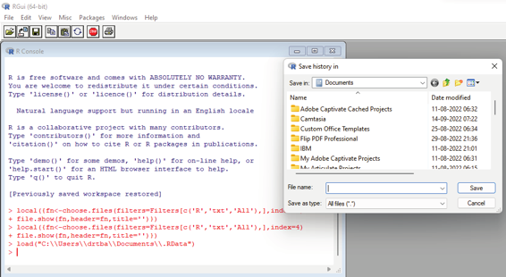
Image showing file browser window opening up on clicking Save History submenu under File menu. The user can assign a name for the file and save it. Default folder that opens is Documents.
Change dir...:
This menu on choosing opens up the file browser presenting the user with the option of changing the default working directory where the various R objects and scripts are stored.
Print:
Using the Print submenu from the File menu the user can print out the contents of the Console. If desired the contents of the console can also be printed out as a PDF.
R Programming in Statistics


Save to File:
This submenu can be used to save the entire session as a file. This will ensure that the user has the option of continuing from the previous session on opening the software the next day.
Exit:
On clicking this submenu, the software can be made to exit. Before exiting the software gives the user the option of saving the session.
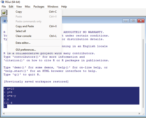
Image showing Edit menu and its various submenus
Prof. Dr Balasubramanian Thiagarajan
37


In the Edit menu the following submenu can be seen:
Copy
Paste
Paste commands only
Copy & paste
Select all
Clear console
Data Editor
Gui prefrences
Copy / Paste menu can be used to copy console contents and paste them. One can choose paste commands only to paste only the commands into the console. Copy and paste menu can be chosen to do both job in one go.
Select all submenu ensures all the contents of the R console selected.
Clear console submenu clears the contents of the console.
Data Editor:
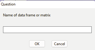
This submenu is used to edit data frame or matrix. On clicking the Data Editor submenu a window will open asking the user for the file name of the data frame / matrix that needs to be edited.
Image showing the dialog box that prompts the user to key in the name of the data frame or matrix that needs to be edited.
R Programming in Statistics


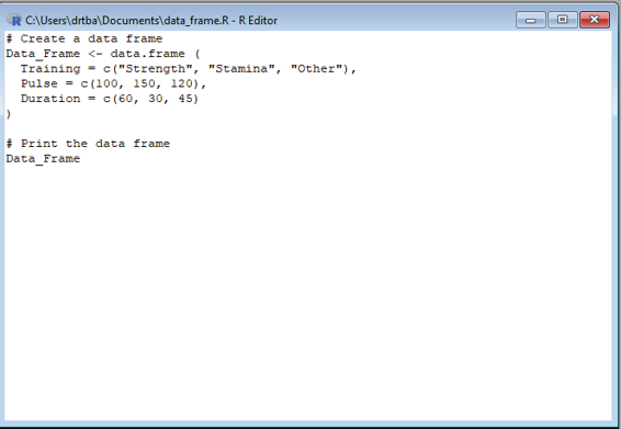

Image showing the Data editor opening after the file name of the data frame is keyed in. Using this interface data can be edited.
GUI Preferences:
This submenu opens up GUI preferences window where T console GUI settings can be manipulated. Default settings of RGUI are ideal for a normal user.
Default settings include:
Single or multiple - MDI MDI toolbar
Pager style - Multiple windows
Font - courier New True type. Size 10 with normal style.
Console rows - 20 columns - 71
Console and Pager colors can also be changed from the default white.
Prof. Dr Balasubramanian Thiagarajan
39


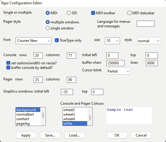

Image showing GUI preferences window.
Single or multiple - MDI is chosen since in this setting R console is displayed with menu at the top. If SDI is chosen only the R console would be opening. In this setting the top menu is not displayed. This setting can be chosen if the user desires an uncluttered environment. For the menu bar to be displayed the MDI toolbar box should be checked. If the user desires the menu to be displayed as a sidebar the MDI sidebar button should be checked instead of MDI toolbar button.
Users commonly change the font type and size to suite their preference. The next setting that is changed is the Console and Pager colors. Console and Pager colors when selected will be displayed in a small preview box. User can visualize the effect of the color settings in the preview box and decide which setting would be appropriate.
View menu:
This menu can be used to control whether the Tool bar and status bar is visible or not. If the user decides to have the Tool bar visible always then in the view menu the Tool bar should be checked. If the status bar is to be viewed then the status bar should also be checked.
R Programming in Statistics


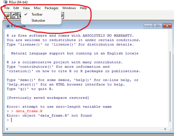

Image showing the Toolbar under view menu is selected so that the menu tools are visible.
Prof. Dr Balasubramanian Thiagarajan
41


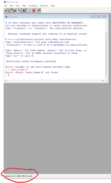

Image showing status bar visible which indicates the version of R
R Programming in Statistics
Under this menu following submenus can be seen listed.
Stop current computation - Clicking on this menu will stop running R code. It would interrupt the code running proces in R. One can perform the same task by pressing on Esc button of keyboard in windows machine.
Stop all computations - This submenu can be used to interrupt all running process in R.
Buffered output - An output buffer is a location in memory or cache where data ready to be seen is held until the display is ready. User can enable this function from Misc menu to ensure that the generated data by R
console is displayed properly. By default this setting is enabled as shown by the tick mark before this submenu. One can choose to disable this action by clicking on the Buffered output submenu which will remove the tick mark. If the same menu is clicked again the setting will get enabled and the tick mark once again appears before this submenu. If this setting is disabled then the result will be displayed almost instantly in the console.
Word completion - This submenu is also listed under Misc menu and is enabled by default. This will ensure that when the commands are keyed into the console by the user the syntax will be auto completed. This is a rather useful setting that helps the user to save considerable amount of coding time.
File name completion - This submenu is also listed under Misc. This again is a useful tool that automatical y completes the file name when the user is keying it partial y. This setting is also enabled by default and saves a lot of coding time.
List objects - This submenu setting on being clicked lists all the objects in the console.
Remove all objects - This submenu when selected will remove all objects from the console.
List search path - Clicking on this submenu will list pathway of various tools and methods that can be searched.
Packages menu:
This menu contains the following submenu:
Load package - This menu can be used to load installed statistical packages and tools. If the user needs to use any package / statistical tool then they must first be loaded to the programming software. Without loading it is not possible to use the features of the package. When the package loads it also loads along with it the relevant libraries and help files to make the life of user that much comfortable. It should be stated that the sheer number of packages available could be mind boggling for the user. Many of them may not be needed for them. It is always better to install and load only the packages that are needed. There could be more than one package for performing the same function. User should be careful enough to install only those packages that are useful for their work.
Prof. Dr Balasubramanian Thiagarajan
43


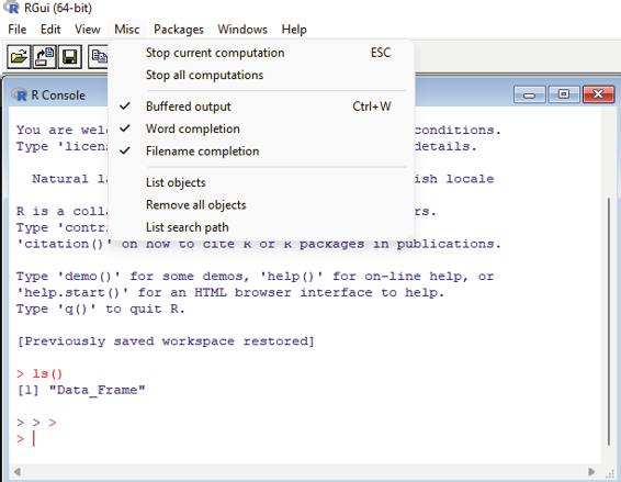


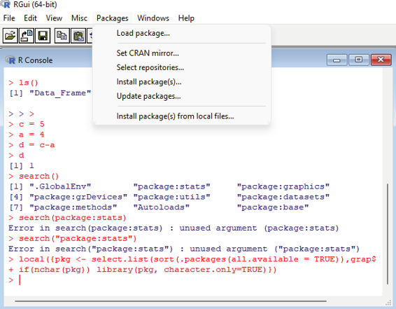

Image showing submenus listed under Misc menu
Image showing the Package menu along with its submenu
R Programming in Statistics


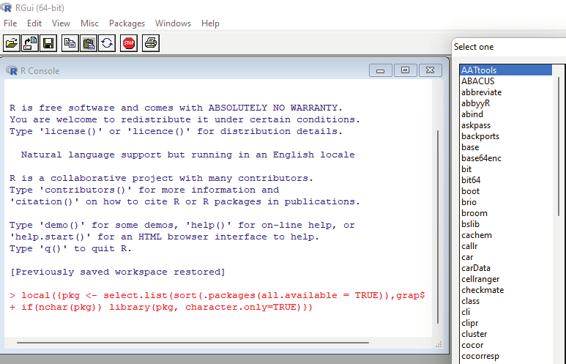

Image showing the list of installed packages that appears when the Load package submenu is clicked Set CRAN Mirror - This submenu allows the user to set the mirror from which pacakges can be downloaded.
The user will have to choose from the list of servers. It is ideal to choose the server that is nearest to the user so that the speed and reliability could be ideal.
Select Repositories - This submenu allows the user to select from the available Repository from which packages and other softwares can be downloaded. A repository is a central place to keep resources that the suers can pull from when necessary.
Install Packages - This submenu when clicked helps the user to install packages for R. On clicking this submenu the user will be persented with a choice of secure CRAN mirrors from which download is desired.
From the list the user needs to choose the optimal server. On choosing the optimal secure CRAN server the user will be presented with a list of R packages that are available for download. Download and instal ation will begin as soon as the user chooses the desired package and click on the OK button. Progress of the download and instal ation can be visualized in the console.
Update Packages - When this submenu is clicked it will display a list of available updates for the software packages installed. The user can select the packages that needs to be updated and click OK for the update process to begin.
Prof. Dr Balasubramanian Thiagarajan
45


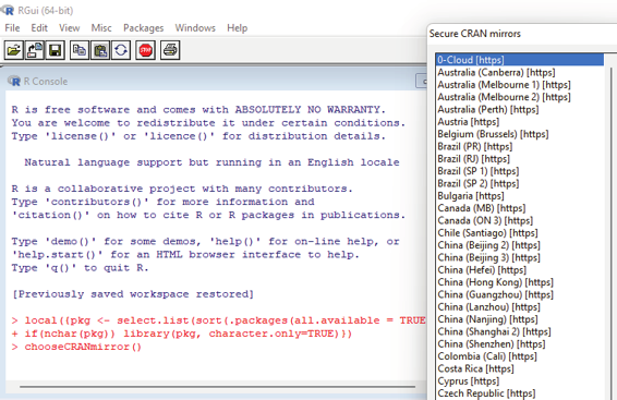


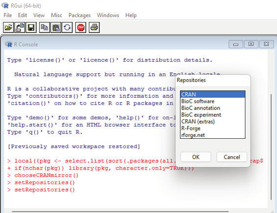

Image showing a list of CRAN mirrors (truncated) from which the ideal one can be chosen by the user. This dialog box appears when the user clicks on set CRAN Mirror submenu Image showing the list of Repositories from where the user can choose the desired one R Programming in Statistics


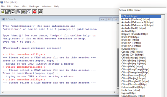


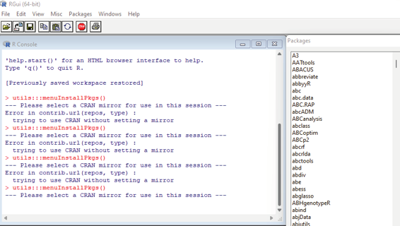

Image showing the list (truncted) list of secure CRAN mirrors from where R packages can be downloaded Image showing the packag list (truncated) from where the user can choose the desired one Prof. Dr Balasubramanian Thiagarajan
47


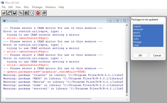

Image showing the list of packages for which updates are available Install Package(s) from local File - This submenu when selected will facilitate the user to install downloaded package from a location in the hard disk.
Windows Menu :
This menu on clicking will reveal the following drop down submenus.
Cascade - If this is clicked the R console will assume less screen space.
Tile Horizontal y - If this is clicked the R console will occupy more horizontal screen space. The console window will enlarge horizontal y.
Tile Vertical y - If this is clicked the R console will occupy more vertical screen space. The console window would enlarge vertical y.
Arrange icons - This submenu will allow the user to rearrange icons that are present above the console window.
R Programming in Statistics


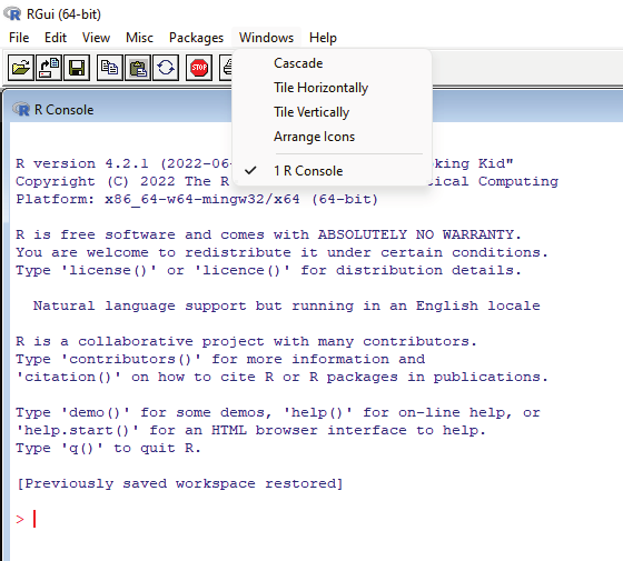


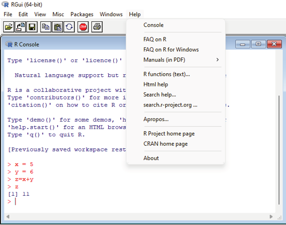

Image showing submenus under Windows menu
Image showing submenu listed under Help menu
Prof. Dr Balasubramanian Thiagarajan
49


Help Menu:
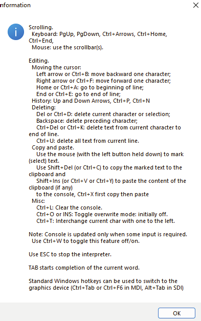
Under this menu various help sources and files are listed. Submenu under this main menu include: Console - When this submenu is clicked it opens up a window containing help pertaining to Console features. It includes keyboard shortcuts for various functions of the console.
Image showing help tips pertaining to Console
R Programming in Statistics


FAQ on R - This submenu when clicked will take the user to a webpage diplaying a set of Frequently asked questions on R and their responses.
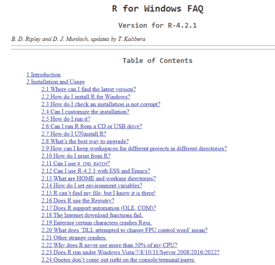
FAQ on R for windows - This submenu on being clicked will take the user to a webpage containing various frequently asked questions pertaining to R software in windows.
Image showing R for windows FAQ web page that gets dsiplayed when this submenu is clicked Prof. Dr Balasubramanian Thiagarajan
51


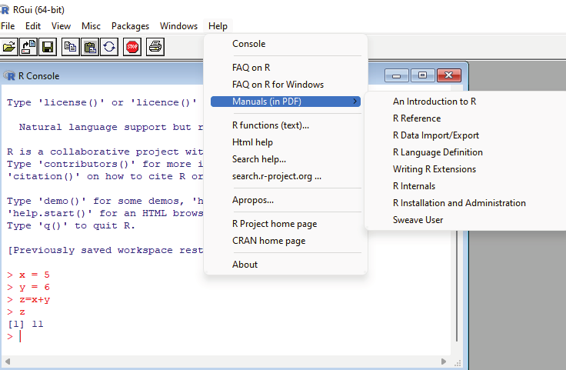


Manuals in (PDF) - On clicking this submenu user will be presented with the choice of links to various manuals for better understanding of R.
Image shwoing various manuals listed under Manuals submenu.
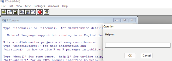
R Functions (Text) - This submenu when selected opens up a search box where the user can key in the desired function and search for help.
Image showing R Functions (Text) menu
R Programming in Statistics


HTML Help - This submenu when clicked displays to the user help files in HTML format.
Search Help - This submenu helps the user to search for relevant help files pertaining to the use of R software.
Search r-Project-.org - This submenu helps the useer to look for resources in r project.org webpage.
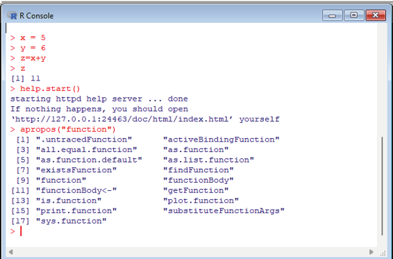
Apropos - This submenu is a function in R that is used to return a character vector with the names of the objects matching of containing the input character partial y.
Image displaying results for the key word ‘function’ keyed into the apropos box.
Prof. Dr Balasubramanian Thiagarajan
53
This is an integrated development environment (IDE) for R. It has a console, syntax-highlighting editor that supports direct code execution, and tools for plotting, history, debugging and workspace.
Features of R Studio IDE:
1. One can access RStudio local y.
2. It has syntax highlighting, code completion and smart indentation features.
3. Content changes can be viewed in real-time with the visual markdown editor.
4. R help is tightly integrated to R Studio.
5. It has interactive debugger to diagnose and fix errors.
6. It also has extensive package development tools.
7. It has dedicated project folders to keep everything organized.
Unique feature of RStudio is that it is tightly integrated with R programming software (base software). It provides the user with full featured IDE experience and nifty GUI. It should be stressed at this point that RStudio should be installed after installing R. Instal ation of both these softwares have already been covered in previous chapters. Ideal y R programming software should be installed before installing RStudio software.
Getting started:
When R studio opens for the first time R will also be launched as wel . It will display three boxes. During the coding phase RStudio will have four different windows. If the 4th window is not visible on the first run all the user needs to do is to click on File/New file/Rscript. The interface will add the 4th block. Background color of all these boxes will be white to start with, it can be changed to user’s preference if desired. As soon as RStudio opens up the user will be confronted with a lot of different windows, each with some tabs. This could be overwhelming for the first ime user. It is easy to get used to it.
Plain text editor - This is like Notepad. “Plain text” means that no fonts, formatting etc as in word processor.
Multiple files can open at once and they appear in tabs. All files can be edited using plain text editor. This can also be used as a script editor. This window can be used to write R code. The main advantage of writing code in this window is that it can be saved and the coding process could be continued in subsequent sessions.
This is not possible if scripts are keyed into the console window. Scripts can be used in the console window only to run it and see the output.
R Programming in Statistics


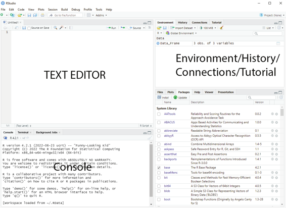

Image showing RStudio interface. Note four compartments. They have been named for convenience by the author.
Default tab in the lower right window is a basic file browser. One can open, delete and rename files there. It is not that well-developed as the operating system’s file browser. It is available to help users managing files without switching to other applications that manage files. Rest of the tabs present in this window include (Plots, Packages, Help and viewer).
Packages tab is the next tab seen in the lower right window. This lists out the various installed packages. If the desired package is selected by placing a tick mark in the box in front of the package the same will be loaded into the program.
Plots tab is the third tab seen in this window. When data is formatted in the form of plots the same will be displayed in a window that appears when clicking on this tab.
Help is the next tab. On clicking this tab a window will open displaying help files. User can search for help using this tab.
Prof. Dr Balasubramanian Thiagarajan
55


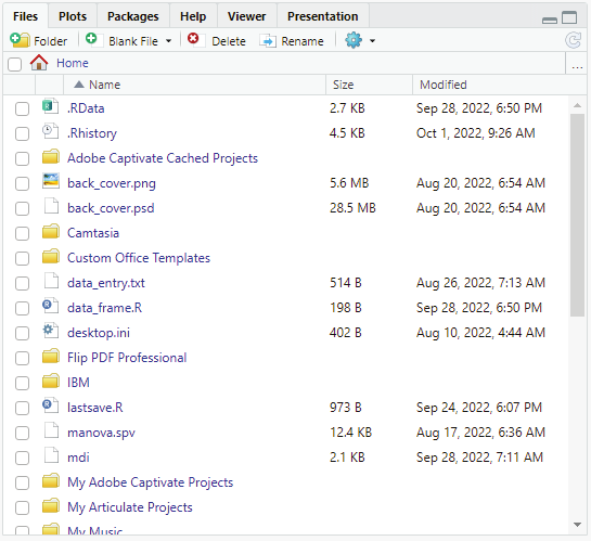

Image showing basic file browser in the lower right window
Viewer - This is the next tab. On clicking this tab a window will open displaying graphs and charts of the data analysed.
Presentation - This is the last tab. RStudio can also be used to create powerful presentations. The created preseentations gets displayed in the window that appears when this tab is clicked.
Console:
This is a tab in RStudio where the user can run R code. The window pane where the console is located contains three tabs:
Console
Terminal
Jobs
When RStudio is run the console contains information about the version of R the user is working with. Console can be used to test the code immediatly. When an expression like 1+3 is entered one can immediatly see the answer output on pressing the Enter key.
R Programming in Statistics


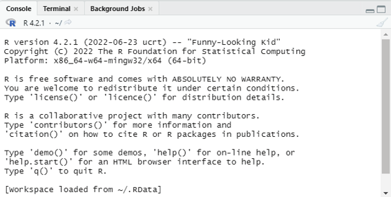


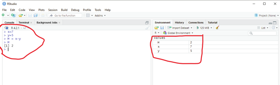

Image showing Console window. It has three tabs. Console, Terminal, and Background jobs Image showing Console window where code is keyed in. In the environment window the values assigned to each letter (variable) can be seen.
Code entered: > x=7
> y=5
> M = x-y
> M
[1] 2
Prof. Dr Balasubramanian Thiagarajan
57


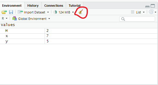

In the code entered x is assinged a value of 7, while y is assigned a value of 5. M is assigned a value of (x-y).
Calculated value of M is 2.
Image showing Environment window where objects are visible. Values of all the three alphabets (variables) can be seen. The window can be cleared of these variables by clicking on the broom icon (red circle).
File menu of RStudio has the following submenu:
New file - This menu allows the user to create new file. It has various submenu which include: RScript - This will create an environment which can be used by the user to create a new script using R programming.
Quarto document - This is a multi-language, next generation version of R Markdown from RStudio, with many new features and capabilities. Like R Markdown, Quarto uses Knitr to execute R code. This document can include a variety of output types like Executable code block, plots, tabular output from data frames and plain text. To use Quarto with R the user will have to install rmarkdown R package. Instal ation of packages in R using RStudio will be discussed. This document can be rendered in HTML, PDF or word.
Quarto presentation - Quarto engine can be used for creating presentations in a variety of formats that include:
revealjs (HTML)
pptx (PowerPoint)
beamer Beamer (LaTeX/PDF).
R Programming in Statistics


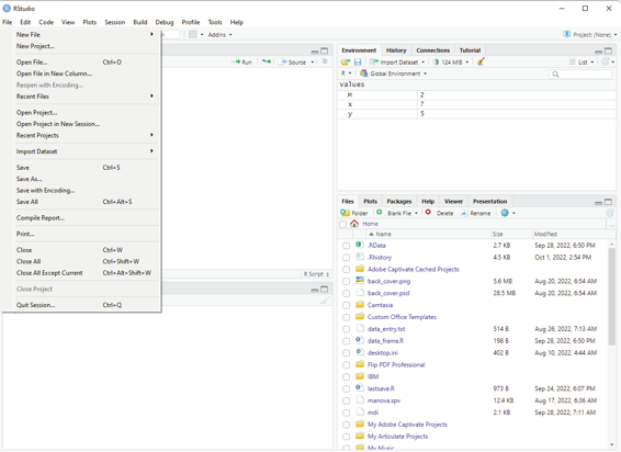

Image showing the File menu of RStudio
R Notebook - This is a R Markdown document that allows for independent and interactive execution of code chunks. It can be considered as a unique execution mode for R Markdown documents and any R Markdown document can be used as a notebook, and all R Notebooks can be rendered to other R Markdown types.
R Markdown - This provides an authoring framework for data science. One can use a single R Markdown file to both
Save and execute code
Generate high quality reports that can be shared.
These documents are ful y reproducible and support dozens of static and dynamic output formats.
Shiny Web app - This is a R package that makes it easy to build interactive web apps from R. Using this one can host standalone apps on a webpage or embed them in R Markdown documents or build dashboards.
These applications can be extended using CSS themes, htmlwidgets and javaScript actions.
Prof. Dr Balasubramanian Thiagarajan
59


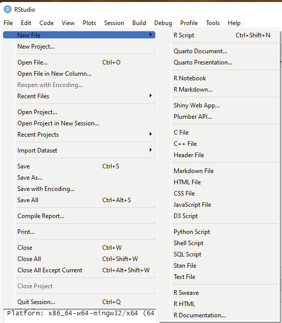

Image showing various submenu listed under New file menu
The user will have to install the Shiny package.
This can be installed by opening an R session and running the followind code: install.packages(“shiny”)
R Programming in Statistics
Plumber API - This allows the user to create a web API by just decorating the existing R source code with roxygen2 - like comments. These comments allow plumber to make the R functions available as API end-points.
C file - R programming tool can be used to create C code. In order to complie c/C++ code R requires installation of additional build tools.
C++ file - R programming tool can be used to create C++ code. R needs to install some additional build tools for this function.
Header files - This can be used together with raster binary files to read data in other applications. Some additional C libraries need to be installed for creation of this file.
Markdown file - This menu can be used to create R Mark down file. Markdown is a simple formatting syntax for authoring HTML, PDF, and MS word documents.
HTML file - Using this submenu the user can create a HTML file.
R Programming software can also be used to create:
Javascript
D3 script
Python script
Shell script
SQL script
Stan file
Text file.
These scripts and files can be created by clicking on the relevant submenu listed under New submenu under File menu.
R Sweave - This is a function in the statistical programming language R that enables integration of R code into LaTeX documents. The main purpose of this feature is to create dynamic reports that can be automatical y updated if data or analysis changes. Sweave document can be created by clicking on the submenu R
Sweave listed under New submenu.
R HTML - R Programming can be used to create HTML files with R code embedded in it. This is known as R HTML. The user can invoke this feature by clicking on the R HTML submenu.
R Documentation - Document that is prepared using the features available in R. The file goes under the term R Documentation. User who prefer to create document in R Document format can click this submenu and a template will be displayed. The document can be created following the displayed template.
Prof. Dr Balasubramanian Thiagarajan
61


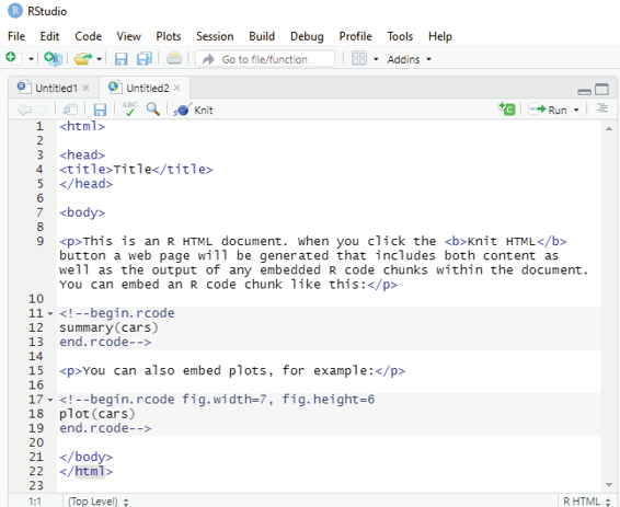

Image showing R HTML template document which gets displayed when the R HTML submenu is clicked Edit Menu - This menu that is available at the top of R Studio window can be used to perform various edit functions. The submenu available under this menu include:
Back
Forward
Undo
Redo
Cut
Copy
Paste
R Programming in Statistics
Paste with Indent - This submenu allows the user to get correct indentation while pasting the R code.
Folding - Has 4 subemnus under it. The source pane in RStudio IDE supports both automatic and user-defined folding of regions of code. Code folding allows the user to easily show and hide code blocks to make it easier to navigate the source file and focus on the coding task at hand.
Foldable regions:
The following types of code regions are automatical y foldable within RStudio:
. Braced regions
. Code chunks within R Sweave or R Markdown documents
. Text sections between headers wtihin R Markdown documents
. Code sections
1. Col apse
2. Expand
3. Col apse Al
4. Expand Al
Go to Line
Find
Find Next
Find Previous
Use Selection for find
Replace and Find
Find in File
Check spelling
Word count
Clear Console
Majority of these submenu are self explanatory.
Prof. Dr Balasubramanian Thiagarajan
63


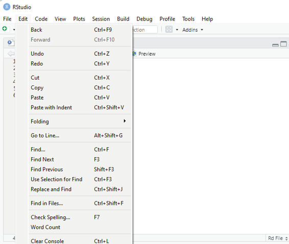

Image showing submenu listed under Edit menu
Code Menu:
Code menu contains the following Submenu:
Go To File/Function
Soft Wrap Long Lines - Enabled by default
Rainbow Parentheses - This setting will replace other types of brackets Terminal
Source File
R Programming in Statistics


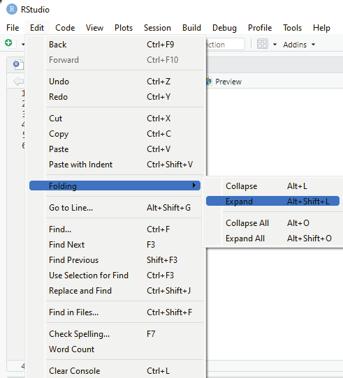

Image showing Submenu under Folding menu
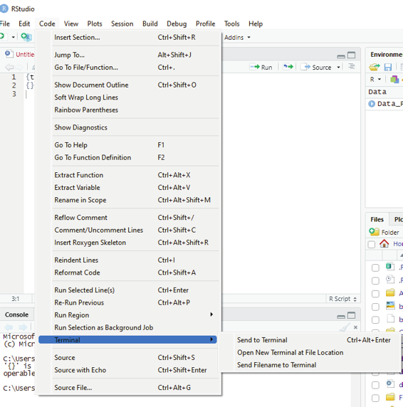
Code Menu also provides submenu that can be clicked to run the code either ful y or from a selected point.
A code from the code window can be selected and their exact function can be extracted using Extract Function Submenu. Similarly variables from the selected code can also be extracted using Extract Variables submenu.
Prof. Dr Balasubramanian Thiagarajan
65


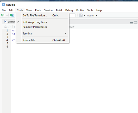

Image showing Code Menu and its various submenu
View menu can be used to hide / unhide tool bar.
Tweak location and number of Panes
Tweak the size of the window by zooming in and out
Switch to a specific tab
Move focus to source
Move focus to console
Move focus to terminal
Move focus to help
Show files
Slow plots
Show viewer
Show environment
Show presentation
Show connections
Show tutorial
Show background jobs
Show other panes
R Programming in Statistics


Prof. Dr Balasubramanian Thiagarajan
67


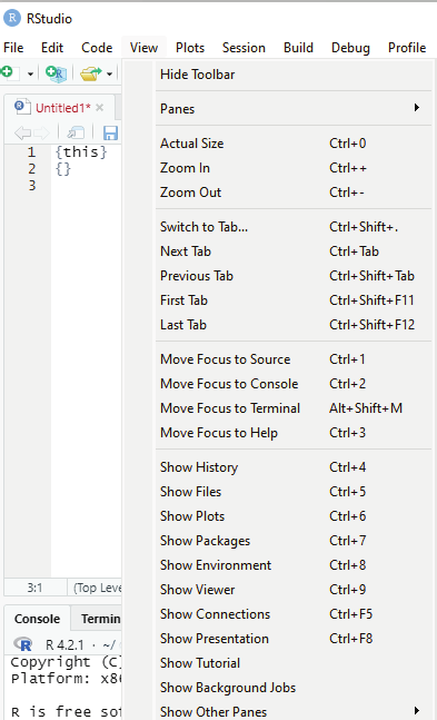

Image showing View Menu and its submenu
R Programming in Statistics


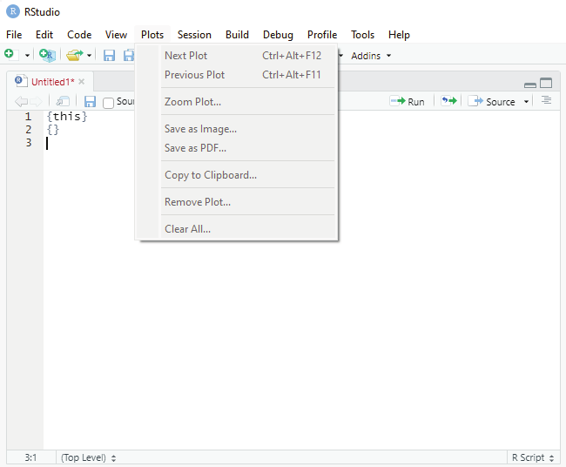

Image showing Plots menu and its submenu
Plots menu - Plots menu can be used to migrate to various plots held in the RStudio.
Debug Menu - This menu is used to debug R code that has been keyed into the console. It runs the code line by line and displays error code thereby helping the user to troubleshoot code errors.
Prof. Dr Balasubramanian Thiagarajan
69


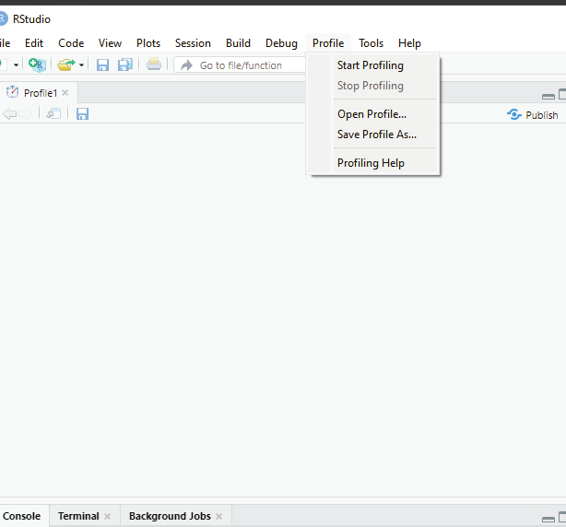

Image showing Profile menu and its submenu
Profiler is a tool that helps the user to understand how R spends its time. It provides an interactive graphical interface for visualizing data from Rprof. This is R’s built in tool for collecting profiling data. Profiler can be run by choosing start profiling submenu from the Menu Profile. The same can be stopped by clicking on Stop Profiling submenu. Help files pertaining to profiling can be accessed by clicking on Profiling Help submenu from Profile menu.
R Programming in Statistics


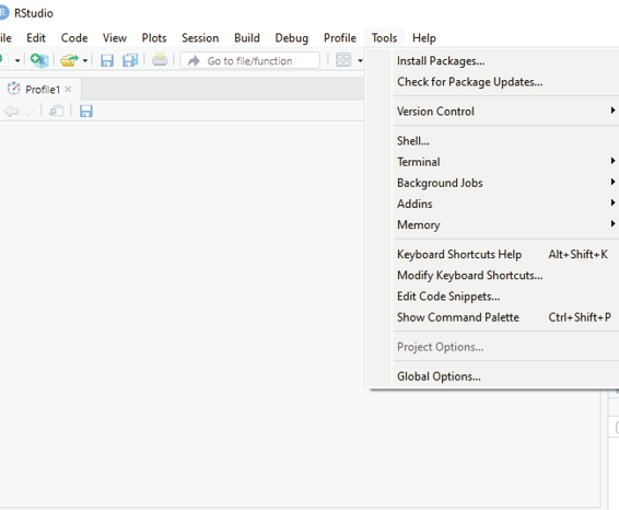

Image showing Tool menu and its submenu
Tools menu:
The following are submenus listed under this menu.
Install Packages - This submenu can be used to install R packages.
Check for Package updates - This submenu can be used to check and install updates for already installed packages if available.
Version control - This submenu helps software teams using RStudio software teams to manage changes to source code over time. Version contol software keeps track of every modification to the code in a special kind of database. If a mistake is made, developers can turn back the clock and comapre earlier versions of the code to help fix the mistake while minimizing disruption to all team members. To make use of this feature the user needs to decide on which control system to use. It can be Git or Subversion. Both of these systems are supported by R. Git or subversion should be installed into the operating system and RStudio restarted for this version control system to work. Version control can be invoked only from a project setup.
Prof. Dr Balasubramanian Thiagarajan
71


Shell - This is also known as a bash or terminal. This program can be used to run other programs, rather than do calculations itself. In windows this menu will open up windows command prompt.
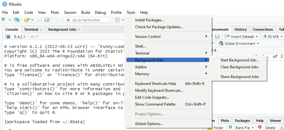
Image showing Background jobs submenu and its various submenus.
Background jobs - RStudio has the ability to send long running R scripts to local and remote background jobs. This functionality can improve the productivity of data scientists and analysts using R since they can continue working in RStudio while jobs are running in the background. Running a Shiny application as a local background job allows the current R session to remain free to work on other things. Three submenus are available under this menu which include:
Start background job - Can be used to start a new background job.
Clear background job - Can be used to clear background jobs View background job - Can be viewed to see running background jobs.
R Programming in Statistics


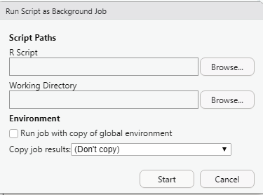

Image showing the dialog box that prompts the user to located the script file that needs to be run in the background. On showing the path to the script file and clicking on the start button the script will be run in the background.
Terminal :
Termial in RStudio provides access to the system shell within the RStudio IDE. Uses of Terminal window includes, advanced source control operations, execution of long running jobs, remote logins, and interactive full scree terminal applications (text editors, terminal multiplexers).
Submenu under terminal include:
New terminal - If this submenu is clicked new terminal window will open.
Go to Current Directory - clicking on this submenu takes the user to the current working directory.
Rename Terminal - User can open more than one terminal window for working. When more than one window it would cause confusion to the user. This submenu provides flexibility to the user to rename the Terminal. By default Terminal window will be suffixed by numbers like (1,2, 3 etc.,) To avoid confusion if more than one terminal is created by the user then it should be renamed.
Prof. Dr Balasubramanian Thiagarajan
73


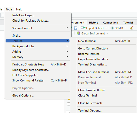

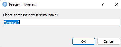
Image showing Terminal submenu along with its submenu
Image showing Rename Terminal window
R Programming in Statistics


Copy Terminal to Editor - Contents of the terminal can be directly copied to the Editor window by clicking on this submenu.
Terminal Diagnostics - This submenu can be used to retrieve details about Terminal windows. It provides details about number of terminal windows open etc., It also provides information about the system.
Move Focus to Terminal - This submenu on being clicked moves focus to the terminal window.
Previous Terminal - Clicking on this submenu will open the previous terminal window if there are more than one terminal opened up.
Next Termial - Clicking on this submenu will take the user to the next terminal.
Clear Terminal Buffer - This submenu will clear the contents of the terminal.
Close Terminal - This submenu closes the Terminal window that is in focus.
Close All Terminals - This submenu when clicked closes all the terminals created.
Image showing Terminal options window
Prof. Dr Balasubramanian Thiagarajan
75
---------------------------
Loaded TerminalSessions: 2
Handle: '6F1B2D42' Caption: 'Terminal 1'
Handle: 'EAFDFBAC' Caption: 'Terminal 2'
Terminal List Count: 2
Handle: '6F1B2D42' Caption: 'Terminal 1' Session Created: true Handle: 'EAFDFBAC' Caption: 'Terminal 2' Session Created: true Global Terminal Information
---------------------------
Caption: 'Terminal 2'
Title: ''
Cols x Rows '87 x 21'
Shell: 'Command Prompt'
Handle: 'EAFDFBAC'
Sequence: '2'
Restarted: 'false
Exit Code: 'null'
Full screen: 'client=false/server=false'
Zombie: 'false'
Track Env 'false'
Local-echo: 'false'
Working Dir: 'Default'
Interactive: 'Always'
WebSockets: 'true'
System Information------------------
Desktop: 'true'
Remote: 'false'
Platform: 'Windows'
Connection Information
----------------------
2022/10/4 14:50:34: Connect WebSocket: 'ws://127.0.0.1:5950/terminal/EAFDFBAC/'
2022/10/4 14:50:34: WebSocket connected
Local-echo Match Failures
-------------------------
<Not applicable>
Image showing Terminal Diagnostics window
R Programming in Statistics


Terminal Options: This submenu will open up window where Options pertaining to terminal can be set.
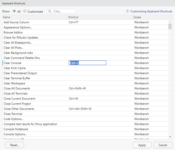
Keyboard shortcut help - This submenu on being clicked opens up keybaord shortcut help. This opens up a window showing various keyboard shortcuts that can be used in RStudio.
Modify keyboard shortcuts - Using this submenu the default keyboard shortcuts can be modified.
Image showing keyboard shortcut change window
Prof. Dr Balasubramanian Thiagarajan
77


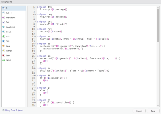

Edit Code Snippets - Code snippets are text macros that are used for quickly inserting common code snippets. If a snippet is selected from the completion list it will be inserted along with several text placeholders which can be filled by the user by typing and then pressing tab to advance to the next placeholder. The pre-saved code snippets can be edited by the user using this submenu.
Image showing Code snippet edit window where code snippets can be edited Global options submenu - This submenu on being clicked opens up Global options window where various settings of RStudio can be changed.
Help:
This menu provides all help files of RStudio under one menu for the benefit of the user.
R Programming in Statistics
Types of Data in R
In any programing language the user needs to use various variables to store various information. Variables are nothing but reserved areas in memory locations to store values. When one creates a variable, some space is reserved in the memory module.
The user can store information of various data types like character, wide character, integer, floating point, double floating point, Boolean etc.
Character - Includes letters, numerical digits, common punctuation marks and whitespace.
Wide character - is a character datatype that is general y greater than the traditonal 8-bit character.
Integer - Is a numerical data.
Floating point - This is a positive or negative whole number with a decimal point.
Double floating point - This is a number format occupying 64 bits in computer memory. A double floating point can hold up to 15 digits.
Boolean - This is actual y a true or false data. This is a system of logical thought that is used to create true/
false statements. This is also known as Logical type of data.
In R, there are 6 basic data types:
Logical - Logical data type in R is also known as boolean data type. It can have two values: TRUE and FALSE
(all upper case).
Numeric - In R, the numeric data type represents all real numbers with or without decimal values.
Integer - The integer data type specifies real values without decimal points. If suffix L is used it specifies integer data. (186L)
Complex - The complex data type is used to specify purely imaginary values in R. One can use the suffix i to specify the imaginary part.
Character - The character data type is used to specify character or string values in a variable. For example “A”
is a single character and “APPLE” is a string. One can use ‘’ or “” to represent strings.
Prof. Dr Balasubramanian Thiagarajan
79
Raw - A raw data type specifies values as raw bytes. The user can use the following method to convert character data types to a raw data type and vice-versa:
charToRaw() - Converts character to raw data
rawToChar() - Converts raw data to character data.
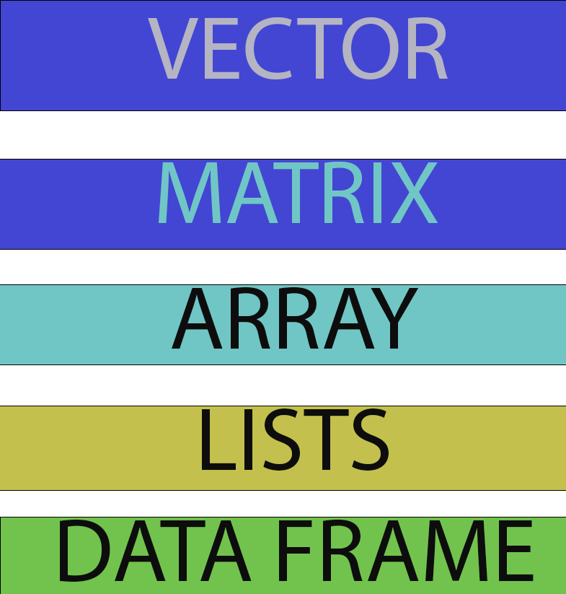
There are basical y 5 different data objects in R that are commonly used. They include: 1. Vector
2. Matrix
3. Array
4. Lists
5. Data Frames
In contrast to other progamming languages the variables in R are not declared as some data type. The variables are assigned with R-Objects and the data type of the R-Object becomes the data type of the variable.
Frequently used types of R-Objects include:
Vectors - Vector is a basic data structure which plays an important role in R programming. In R, a sequence of elements which share the same data type is known as a vector. A vector supports logical, integer, double, character, complex or raw data type. Elements contained in vector are known as components of the vector.
The user can check the type of vector with the help of typeof() function.
Length is an important property of a vector. A vector length is basical y the number of elements in the vector, and is calculated with the help of length() function.
Simply stated a Vector is a sequence of data elements of the same basic type.
There are 5 classes of vectors also termed as Atomic Vectors:
* Logical - This type of vector can either take a value of TRUE or FALSE. (Note all these letters should be in upper case).
* Integer - Takes a whole number value. Example (15L, 30L, 4566L). R is capable of handling integers that are fairly long i.e., 32-bit long. Hence, L is used as a suffix after the integer to indicate to R that it is a long integer.
* Numeric - Can take a whole number of a decimal number. Example ( 6, 4.876).
* Complex - R support complex data types that are a set of complex numbers. The complex data type is to store numbers with an imaginary component and hence is suffixed with an ‘i’.
R Programming in Statistics


* Character - Single character of a sequence of characters forming a word. This data type should be entered between ‘’ of “” to indicate to the software that the data type is character.
Example ‘A’ “Hello”.
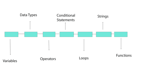
Image showing the heirarchy of R Programming in data analysis What are variables?
Varaible is a reserved memory locations to store values. When the uesr creates a variable some space is reserved in the memory. In lay terms it can be compared to a container that can hold only one material. The type of material can vary. The software identifies the type of data that has been allocated to a variable and allots a suitable memory place to hold on to it. This data is held on to the memory till such time when the user replaces it with another data.
Data types:
This helps in classification of the type of data that is held in a variable. The class or type of the data held in the memory allocated to the variable is important because the size of the memory block allocated varies according to the type of the data contained in the variable. Classification of data type held in the variable is important because it helps in the user in performing different types of opeartions using R Programming language. For example if the data type happens to be numeric then arithmetic calculations, logical operations and string operations can be performed using R programming software. These same operations cannot be performed if the variable holds a character data. When one considers vector as a whole, either one can have a single element belonging to one of the above described data types or it can be a sequence of elements.
Prof. Dr Balasubramanian Thiagarajan
81
x = 15
x=15
y <- "Hello"
y = “Hello”
True -> B
B =TRUE
Image showing three variables and their values coded. Variable x has been assigned a value of 15, numeric variable. variable y has been assigned a value of “Hello” a character variable and Variable B has been assigned a boolean value of TRUE.
Image showing 5 different data types used in R Programming
R Programming in Statistics


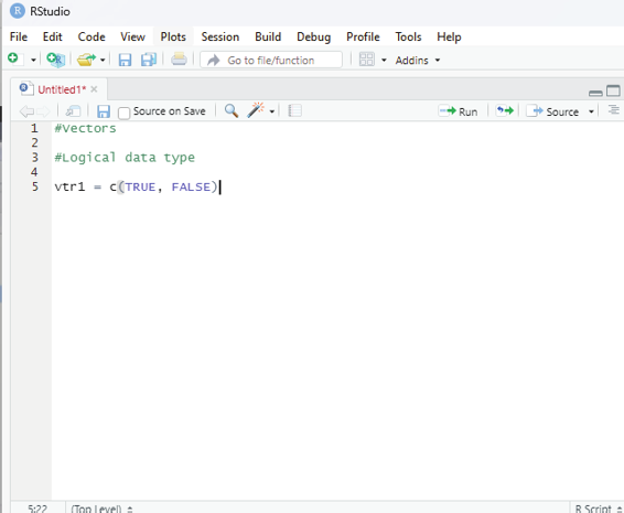

In order to demonstrate the various data types in R, one has to open the R studio. The scripting area should be used to key in the scripts. This is a must when the user needs to write multiple lines of code. The console area can be used to execute a single line of code. Every time the user declares a variable it gets automatical y updated in the Gobal Environment window.
Image showing code entered into scripting window. After entering the code it can be run on clicking the Run button. The output will be displayed in the console window.
Prof. Dr Balasubramanian Thiagarajan
83


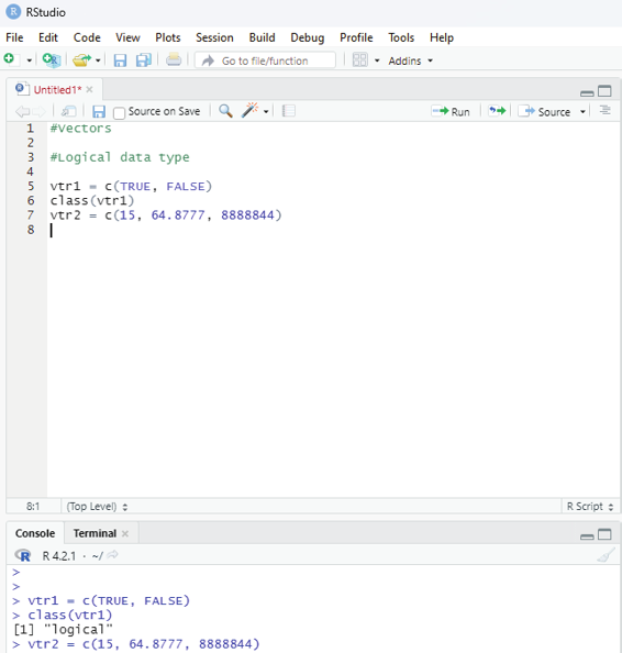
#Vectors
#Logical data type
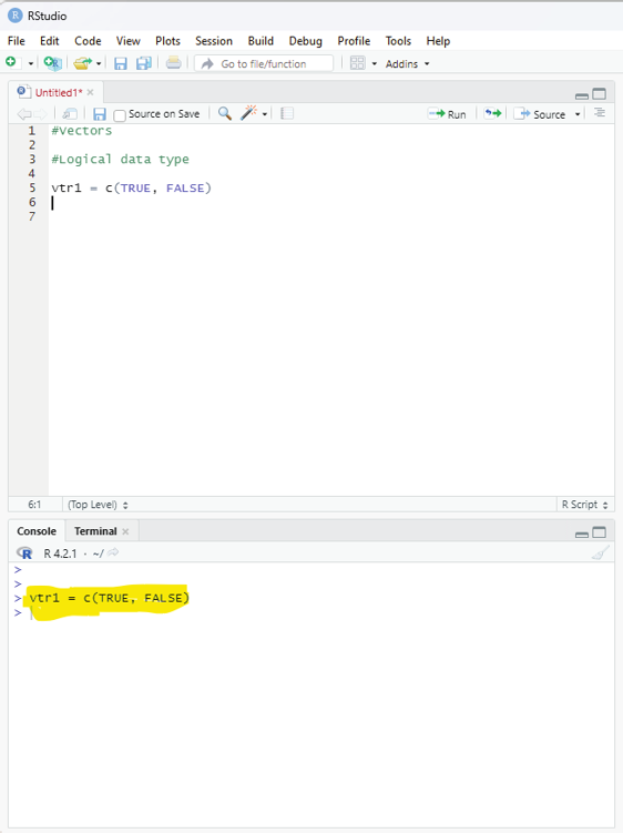
vtr1 = c(TRUE, FALSE)
Note the code block above. This code block can be used to allocate variables to a vector. In this code name of the vector is given as vtrl1 and the variable stored is of logical type (TRUE, FALSE). They should be in capital letters. Anything that is typed after # is not run by R. They will be considered as a comment.
Image showing the result of clicking the run button. The result of running the code is displayed in the console window (highlighted yellow).
In order to ascertain what type of data has been allocated to the variable the class command would help.
Syntax for ascertaining the data type associated with a variable is: class(name of the variable) R Programming in Statistics


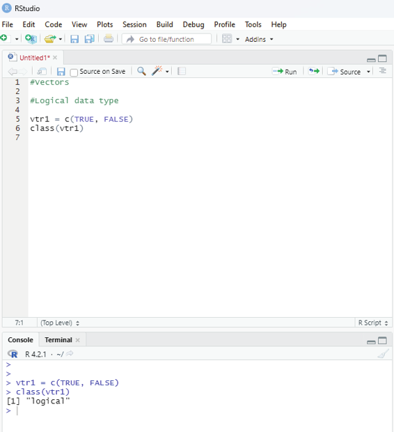

Image showing command to ascertain the category of variable inside vector named vtr1. Note the output of the code run in the console window.
Prof. Dr Balasubramanian Thiagarajan
85


class(vtr1)
Output: [1] “logical”
Another vector is created. Name assigned to the newly created vector is vtr2.
vtr2 = c(15, 64.8777, 8888844)
In the newly created vector named vtr2 has the following data allocated to it; 15
64.8777
8888844
On pressing the run button in the scripting window the script is run and the output is displayed in the console window.
Image showing the second vector created and values alloted. Result is displayed in Console window R Programming in Statistics


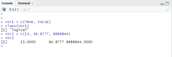


Values assigned to a vector can be seen by just keying the name of the vector in the console window and pressing the Enter key. For example the vale stored in the vtr2 can be ascertained by keying in vtr2 in console window and pressing the Enter key.
Image showing the console window where a command to display value stored in vector 2 (vct2) is displayed.
Note the value is different from that of what was keyed in the scripting window. This is because one assigned value has four decimals and hence all the whole numbers are converted into decimals by adding four zeros after the whole number.
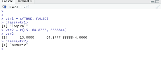
When the code for identifying the data type of vct2 is keyed in the output displays Numeric.
Image showing the result of commad class(vtr2). Type of data stored in the variable is displayed as numeric Prof. Dr Balasubramanian Thiagarajan
87


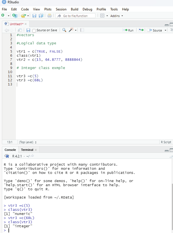

Example for integer type data stored in a vectar. If the user desires to store a value 0f 5 in a vector titled vtr3
then the class statement will describe the data as Numeric. If the stored number (whole number) is suffixed with ‘L” then the class statement decribes the data as an integer.
Image showing Integer class stored in a vector. Note only when the stored whole number is suffixed with a
“L” the value will be recognized by R as an Integer. Note the console command class(vtr3) and its result.
R Programming in Statistics
#This code is entered into the scripting window and run button is clicked.
The console window shows the result as being the value 5 assigned to the variable titled vtr3.
In the console window the following script is entered and run: class(vtr3)
When the above command is keyed into the console window and run the result is displayed as:
[1} “numeric”
If the whole numer entered into a variable is suffixed with “L” then it is considered as an Integer by R.
vtr3 c=(68L)
The above code is entered into the scripting window and run. This displays the result that the number 68L
has been stored in the variable named vtr3.
class(vtr3)
The above command is given in the console window and run. This displays a class value as “Integer”.
What will happen to the class if three types of variables included in a vector?
Code:
vtr5 = c(TRUE,35L,3.14)
vtr5 contains three types of variables:
1. Logical data
2. Integer
3. Numeric
Prof. Dr Balasubramanian Thiagarajan
89


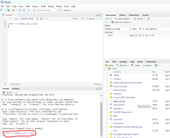

Image showing three types of data entered into a vector. The first one is the logical vector, the next one is an integer and the third one is the numeric. This code is entered into the scripting window. On clicking the run button the console window will demonstrate all these three data.
In the console window the following code can be used to ascertain the class of data: class (vtr5)
On clicking the enter button the console displays as numeric the type of data.
R Programming in Statistics


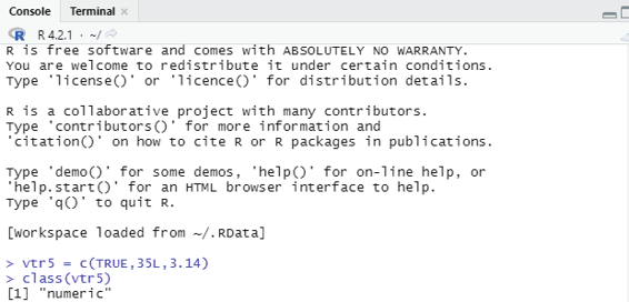


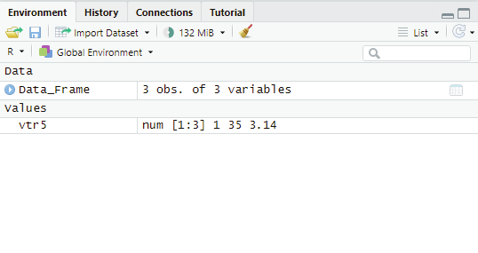

Image showing the console window when class query is used. It displays numeric as the type of data.
Image showing the Environment window where the name of the variable vtr5 is displayed and the class is displayed as numeric (num). It also says that there are three data (1:3) in the variable. Note 1 is used to instead of TRUE. Logical value TRUE has been assigned the numeric value of 1. When multiple types of data is entered into a vector, R software convers them into a unified data.
Prof. Dr Balasubramanian Thiagarajan
91


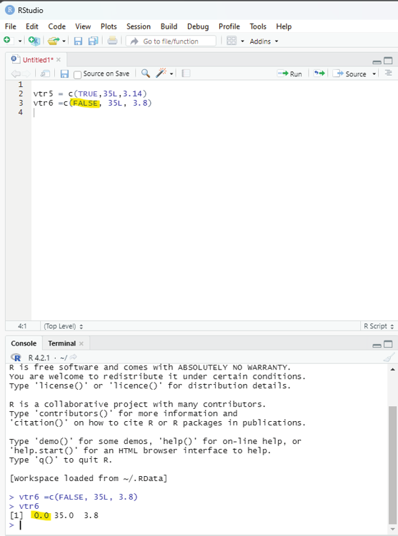

Now let us see what value would R assign if FALSE is used instead of TRUE: The logical value of FALSE is assigned a value of 0 by R as shown in the image below.
R Programming in Statistics
In this code the first value is Logical, the second is an integer and the third one is numeric. After these values have been assigned to vtr5 then when the class of the vector is queried for using the code class(vtr5). The output generated would be “numeric”. This occurs because R converts all values into numeric data. The Logical data is also converted into numeric data, TRUE is assigned a value of 1. If it would have been FALSE then value 0 would be assigned.
vtr6 = c(“hel o”, FALSE, 50L)
In this example code one can see that vr6 variable contains a character, Logical value and an Integer. On entering this data into the vector these values are created. Console window would reveal that all the data created are within double quotes. R considers all these values to be of character type. In other words it converts both logical and integer values to be character type. When different data types are entered into a variable then R converts them into a single data type.
Matrix:
This is quite similar to arrays in other programs. These are R objects in which the elements are arranged in a two dimensional rectangular layout.
Syntax for creating matrix in R:
matrix(data,nrow,ncol,byrow,dimnames)
* data - it is the input vector which becomes the data elements of the matrix.
* nrow - it is the number of rows to be created.
* ncol - is the number of columns to be created.
* byrow - is a logical clue. If true theen the input vector elements are arranged by row.
* dimname - is the names assigned to rows and columns.
code:
mtr = matrix(c(5:29),5,5,)
Using the above code a matrix is created with numbers between5 and 29 with an increment of 1 between them. Number of Rows are specified as 5 and number of columns is specified as 5. This code is entered into the script window of RStudio. On clicking the Run button the values for the matrix get assigned successful y as seen from the output in the console window. On typing mtr (name of the matrix) in the console window and Enter button is clicked. Output demonstrates the arrangement of numbers between 5 and 29 in the form of matrix as shown in the figure.
Prof. Dr Balasubramanian Thiagarajan
93


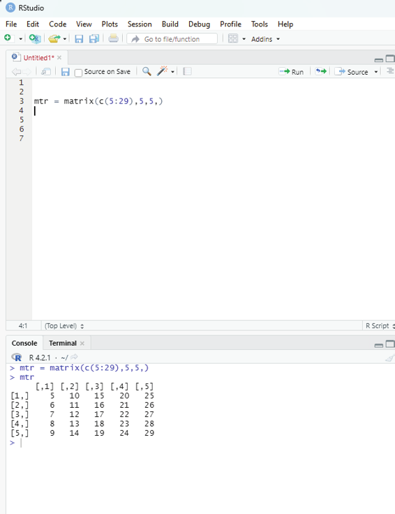

Image showing screen shot of the matrix code which is used to arrange numbers between 5 and 29 in 5 rows and 5 columns matrix
R Programming in Statistics
By default matrices are in column-wise order.
Another code for creating a matrix:
A = matrix(
# Taking sequence of elements
c(1, 2, 3, 4, 5, 6, 7, 8, 9),
# No of rows
nrow = 3,
# No of columns
ncol = 3,
# By default matrices are in column-wise order
# So this parameter decides how to arrange the matrix byrow = TRUE
)
# Naming rows
rownames(A) = c(“a”, “b”, “c”)
# Naming columns
colnames(A) = c(“c”, “d”, “e”)
cat(“The 3x3 matrix:\n”)
print(A)
Creating a matrix where all rows and columns are filled by a single constant “k”.
Note: Use of print command need not be used. It is sufficient to key in the variable name in the console window and pressing the Enter button will display the result. Use of print command or just the name of the variable is a personal choice of the programmer. Print syntax is introduced just to alert the reader that there are more than one way to instruct R to perform a task.
Syntax used is:
matrix(k,m,n)
k-the constant
m-number of rows
n-number of columns
Prof. Dr Balasubramanian Thiagarajan
95


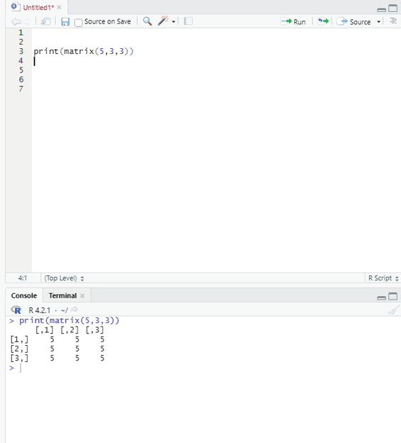

Code:
print(matrix(5,3,3))
On running this code R creates a 3x3 matrix with all values filled as 5.
Image showing matrix filled with the same number i.e., 5
R Programming in Statistics


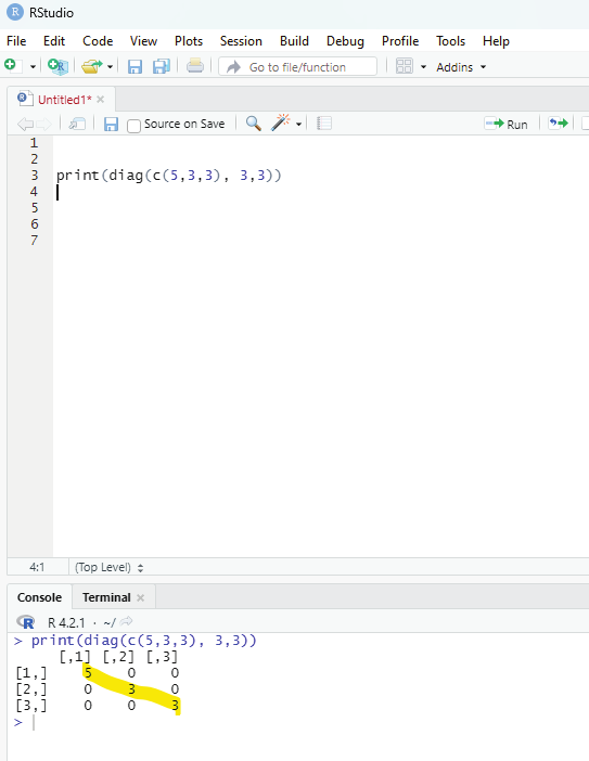

Diagonal Matrix:
A diagonal matrix is a matrix in which the entries outside the main diagonal are 5,3,3.
Code:
#This diagonal matrix should have 3 rows and 3 columns.
# Fil ed by array of elements (5,3,3).
print(diag(c(5,3,3), 3,3))
Image showing a diagonal matrix with numbers 5,3, and 3 in the main diagonal Prof. Dr Balasubramanian Thiagarajan
97


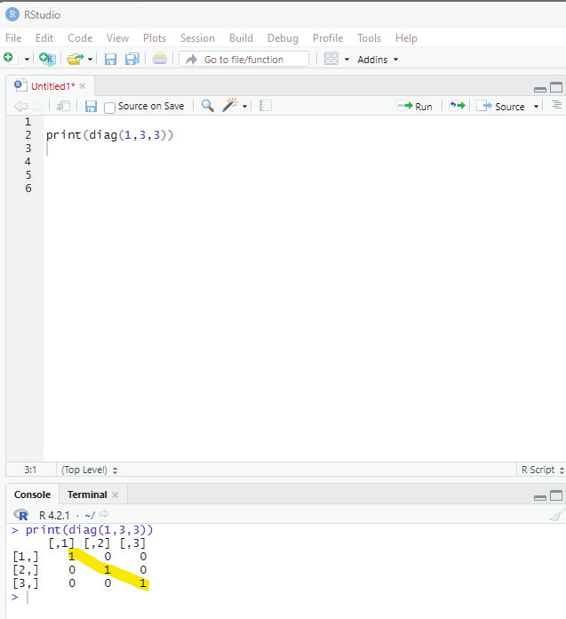

Identity matrix:
A square matrix in which all the elements of the principal diagonal are ones and all other elements are zeros.
To create such a matrix the following syntax should be used: Syntax:
diag(k,m,n)
Parameters:
k:1
m=no of rows
n=no of columns
print(diag(1,3,3))
Image showing the result of code with 1 in the major diagonal and zero in al R Programming in Statistics
Example for a matrix with 2 rows and three columns:
> A = matrix(
+ c(2,4,3,1,5,7), # the data elements
+ nrow=2, # number of rows
+ ncol=3, # number of columns
+ byrow = TRUE) # fill matrix by rows
> A # Print the matrix
These examples help the reader to understand that there are various coding methodologies available in R
Programming and it is for the programmer to choose which is best suited for them.
Assessing various elements in a matrix:
An element at the mth row, nth column of matrix A can be assessed by the expression A[m,n].
> A[2,3] # element at the 2nd row, 3rd column.
The entire mth row A can be extracted as A[m,].
> A [2] # 2nd row.
The entire nth column A can be extracted as A[,n].
> A[,3] # 3rd column
One can also extract more than one rows or columns at a time.
Matrix Construction:
There are various ways to construct a matrix. When one constructs a matrix directly with data elements, the matrix content is filled along the column orientation by default.
Example:
> B=matrix(
+ c(2,4,3,1,5,7),
+ nrow=3,
+ ncol=2)
# B has three rows and two columns
Transpose:
One can transpose a matrix by interchanging its column and rows with the function t.
Prof. Dr Balasubramanian Thiagarajan
99
Combining Matrices:
Columns of two matrices having the same number of rows can be combined into a larger matrix.
> c=matrix(
+ c(7,4,2),
+ nrow=3,
+ ncol=1,
>c #c has 3 rows.
One can combine matrices B and C using cbind command.
> cbind(B, C)
One can also combine the rows of two matrices if they have the same number of columns with rbind function.
> D=matrix(
+ c(6,2),
+ nrow=1,
+ ncol=2)
>D # D has 2 columns
>rbind(B,D)
Deconstruction:
The user can deconstruct a matrix by applying c function which combines all the column vectors into one.
>c(B)
R Programming in Statistics


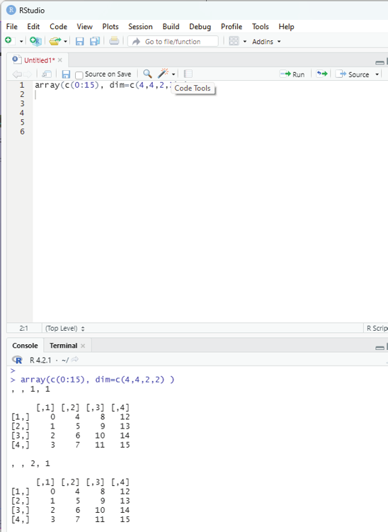

Arrays:
These are R data objects which can store data in more than two dimensions. Only precondition being that the different data should be of the same class.
Syntax used:
array(data,dim,dimnames)
array(c(0:15), dim=c(4,4,2,2) )
Basical y 64 elements are stored in 4 different matrices.
If the number of values is less than the number of arrays / matrix then it takes the same input vector and starts to insert elements already inserted.
Image showing an array with numbers ranging from 0 to 15 created. It has 4 columns, four rows and 4 dimensions
Prof. Dr Balasubramanian Thiagarajan
101
> array(c(0:15), dim=c(4,4,2,2) )
, , 1, 1
[,1] [,2] [,3] [,4]
[1,] 0 4 8 12
[2,] 1 5 9 13
[3,] 2 6 10 14
[4,] 3 7 11 15
, , 2, 1
[,1] [,2] [,3] [,4]
[1,] 0 4 8 12
[2,] 1 5 9 13
[3,] 2 6 10 14
[4,] 3 7 11 15
, , 1, 2
[,1] [,2] [,3] [,4]
[1,] 0 4 8 12
[2,] 1 5 9 13
[3,] 2 6 10 14
[4,] 3 7 11 15
, , 2, 2
[,1] [,2] [,3] [,4]
[1,] 0 4 8 12
[2,] 1 5 9 13
[3,] 2 6 10 14
[4,] 3 7 11 15
Seen above are the four columns and rows arranged in four dimensions.
Two vectors containing similar objects can be combined into one array.
Example:
# Creating two vectors of different lengths.
vector1 <- c(7,5,4)
vector2 <- c(21,11,14,16,22)
# The next step is to combine these two vectors into a single array.
result <- array(c(vector1,vector2), dim= c (3,3,2))
print(result)
R Programming in Statistics


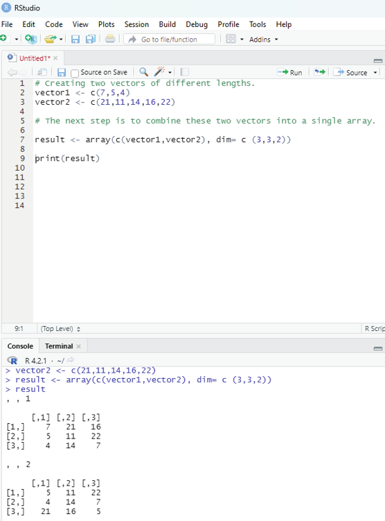

Image showing two vectors with data of different sizes combined into a single array with two dimensions Prof. Dr Balasubramanian Thiagarajan
103
Columns and Rows in array can be named using dimnames parameter.
Example:
# Step 1 - Create two vectors of different lengths.
vector1 <-c(3,4,8)
vector2 <-c(10,13,11,22,34,22)
column.names <-c(“COL1”, “COL2”, “COL3”)
row.names <-c(“ROW1”, “ROW2”, “ROW3”)
matrix.names <-c(“matrix1”, “matrix2”)
# Step 2 - Combine these vectors as input into the array.
result <-array(c(vector1,vector2),dim = c(3,3,2),dimnames=list(row.names,column.names,matrix.names)
print(result)
Note the command list is used here. It will be discussed later in the chapter.
One can assess the elements in the array using the following command:
# To print the third row of the second matrix of the array
print(result[3,,2])
# To print the element in the 1st row and 3rd column of the 1st matrix.
print(result[1,3,1])
# In order to print the entire two matrices.
print(result[,,2])
Manipulating elements within array:
Since array is made up of matrices in multiple dimensions, the operations on elements of array can be carried out by accessing elements of the matrices.
R Programming in Statistics


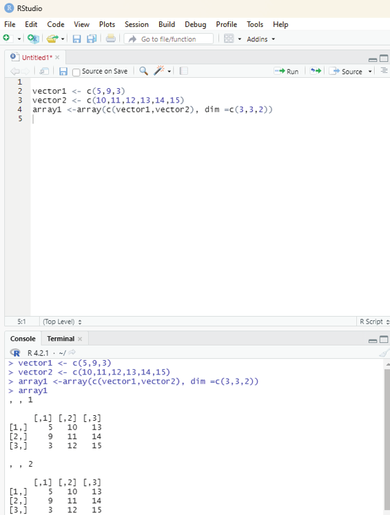

# Create two vectors of different lengths.
vector1 <- c(5,9,3)
vector2 <- c(10,11,12,13,14,15)
# Take these vectors as input into the array.
array1 <-array(c(vector1,vector2), dim =c(3,3,2))
Image showing array1 being generated using the code specified Prof. Dr Balasubramanian Thiagarajan
105


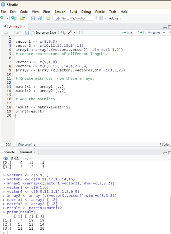

# Create two vectors of different lengths.
vector3 <- c(9,1,0)
vector4 <- c(6,0,11,3,14,1,2,6,9)
array2 <- array (c(vector3,vector4),dim =c(3,3,2))
# Create matrices from these arrays.
matrix1 <- array1 [,,2]
matrix2 <- array2 [,,2]
# Add the matrices.
result <- matrix1+matrix2
print(result)
Image showing the results of adding two matrices
R Programming in Statistics


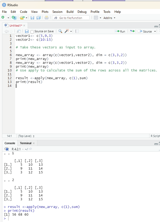

Calculations can be performed across array elements:
One can perform calculations across the elements in an array using the following syntax: apply(x, margin, fun)
x is an array
margin is the name of the data set used
fun is the function to be applied across the elements in the array.
Image showing apply() command used to perform calculations
Prof. Dr Balasubramanian Thiagarajan
107
# Create two vectors of different lengths.
vector1<- c(5,9,3)
vector2<- c(10:15)
# Take these vectors as input to array.
new_array <- array(c(vector1,vector2), dim = c(3,3,2)) print(new_array)
# Use apply to calculate the sum of the rows across all the matrices.
result <-apply(new_array, c(1),sum)
print(result)