Chapter 1: Building Abstractions with Functions by Harold Abelson, Gerald Jay Sussman, Julie Sussman - HTML preview
Download the book in PDF, ePub, Kindle for a complete version.
including 0, None, and the boolean value False. All other numbers are true values. In Chapter 2, we will see
that every native data type in Python has both true and false values.
Boolean values. Python has two boolean values, called True and False. Boolean values represent truth
values in logical expressions. The built-in comparison operations, >, <, >=, <=, ==, !=, return these
values.
22
>>> 4 < 2
False
>>> 5 >= 5
True
This second example reads “5 is greater than or equal to 5”, and corresponds to the function ge in the
operator module.
>>> 0 == -0
True
This final example reads “0 equals -0”, and corresponds to eq in the operator module. Notice that Python
distinguishes assignment (=) from equality testing (==), a convention shared across many programming languages.
Boolean operators. Three basic logical operators are also built into Python:
>>> True and False
False
>>> True or False
True
>>> not False
True
Logical expressions have corresponding evaluation procedures. These procedures exploit the fact that the truth
value of a logical expression can sometimes be determined without evaluating all of its subexpressions, a feature
called short-circuiting.
To evaluate the expression <left> and <right>:
1. Evaluate the subexpression <left>.
2. If the result is a false value v, then the expression evaluates to v.
3. Otherwise, the expression evaluates to the value of the subexpression <right>.
To evaluate the expression <left> or <right>:
1. Evaluate the subexpression <left>.
2. If the result is a true value v, then the expression evaluates to v.
3. Otherwise, the expression evaluates to the value of the subexpression <right>.
To evaluate the expression not <exp>:
1. Evaluate <exp>; The value is True if the result is a false value, and False otherwise.
These values, rules, and operators provide us with a way to combine the results of tests. Functions that
perform tests and return boolean values typically begin with is, not followed by an underscore (e.g., isfinite,
isdigit, isinstance, etc.).
1.5.5 Iteration
In addition to selecting which statements to execute, control statements are used to express repetition. If each line
of code we wrote were only executed once, programming would be a very unproductive exercise. Only through
repeated execution of statements do we unlock the potential of computers to make us powerful. We have already
seen one form of repetition: a function can be applied many times, although it is only defined once. Iterative
control structures are another mechanism for executing the same statements many times.
Consider the sequence of Fibonacci numbers, in which each number is the sum of the preceding two:
0, 1, 1, 2, 3, 5, 8, 13, 21, ...
Each value is constructed by repeatedly applying the sum-previous-two rule. To build up the nth value, we
need to track how many values we’ve created (k), along with the kth value (curr) and its predecessor (pred),
like so:
23
>>> def fib(n):
"""Compute the nth Fibonacci number, for n >= 2."""
pred, curr = 0, 1
# Fibonacci numbers
k = 2
# Position of curr in the sequence
while k < n:
pred, curr = curr, pred + curr
# Re-bind pred and curr
k = k + 1
# Re-bind k
return curr
>>> fib(8)
13
Remember that commas seperate multiple names and values in an assignment statement. The line:
pred, curr = curr, pred + curr
has the effect of rebinding the name pred to the value of curr, and simultanously rebinding curr to the
value of pred + curr. All of the expressions to the right of = are evaluated before any rebinding takes place.
A while clause contains a header expression followed by a suite:
while <expression>:
<suite>
To execute a while clause:
1. Evaluate the header’s expression.
2. If it is a true value, execute the suite, then return to step 1.
In step 2, the entire suite of the while clause is executed before the header expression is evaluated again.
In order to prevent the suite of a while clause from being executed indefinitely, the suite should always
change the state of the environment in each pass.
A while statement that does not terminate is called an infinite loop. Press <Control>-C to force Python
to stop looping.
1.5.6 Practical Guidance: Testing
Testing a function is the act of verifying that the function’s behavior matches expectations. Our language of
functions is now sufficiently complex that we need to start testing our implementations.
A test is a mechanism for systematically performing this verification. Tests typically take the form of another
function that contains one or more sample calls to the function being tested. The returned value is then verified
against an expected result. Unlike most functions, which are meant to be general, tests involve selecting and
validating calls with specific argument values. Tests also serve as documentation: they demonstrate how to call a
function, and what argument values are appropriate.
Note that we have also used the word “test” as a technical term for the expression in the header of an if or
while statement. It should be clear from context when we use the word “test” to denote an expression, and when
we use it to denote a verification mechanism.
Assertions. Programmers use assert statements to verify expectations, such as the output of a function
being tested. An assert statement has an expression in a boolean context, followed by a quoted line of text
(single or double quotes are both fine, but be consistent) that will be displayed if the expression evaluates to a false
value.
>>> assert fib(8) == 13, ’The 8th Fibonacci number should be 13’
When the expression being asserted evaluates to a true value, executing an assert statement has no effect.
When it is a false value, assert causes an error that halts execution.
A test function for fib should test several arguments, including extreme values of n.
>>> def fib_test():
assert fib(2) == 1, ’The 2nd Fibonacci number should be 1’
assert fib(3) == 1, ’The 3nd Fibonacci number should be 1’
assert fib(50) == 7778742049, ’Error at the 50th Fibonacci number’
24
When writing Python in files, rather than directly into the interpreter, tests should be written in the same file
or a neighboring file with the suffix _test.py.
Doctests. Python provides a convenient method for placing simple tests directly in the docstring of a function.
The first line of a docstring should contain a one-line description of the function, followed by a blank line. A
detailed description of arguments and behavior may follow. In addition, the docstring may include a sample
interactive session that calls the function:
>>> def sum_naturals(n):
"""Return the sum of the first n natural numbers
>>> sum_naturals(10)
55
>>> sum_naturals(100)
5050
"""
total, k = 0, 1
while k <= n:
total, k = total + k, k + 1
return total
Then, the interaction can be verified via the doctest module. Below, the globals function returns a representation of the global environment, which the interpreter needs in order to evaluate expressions.
>>> from doctest import run_docstring_examples
>>> run_docstring_examples(sum_naturals, globals())
When writing Python in files, all doctests in a file can be run by starting Python with the doctest command line
option:
python3 -m doctest <python_source_file>
The key to effective testing is to write (and run) tests immediately after (or even before) implementing new
functions. A test that applies a single function is called a unit test. Exhaustive unit testing is a hallmark of good
program design.
1.6 Higher-Order Functions
We have seen that functions are, in effect, abstractions that describe compound operations independent of the
particular values of their arguments. In square,
>>> def square(x):
return x * x
we are not talking about the square of a particular number, but rather about a method for obtaining the square
of any number. Of course we could get along without ever defining this function, by always writing expressions
such as
>>> 3 * 3
9
>>> 5 * 5
25
and never mentioning square explicitly. This practice would suffice for simple computations like square,
but would become arduous for more complex examples. In general, lacking function definition would put us at
the disadvantage of forcing us to work always at the level of the particular operations that happen to be primitives
in the language (multiplication, in this case) rather than in terms of higher-level operations. Our programs would
be able to compute squares, but our language would lack the ability to express the concept of squaring. One of the
things we should demand from a powerful programming language is the ability to build abstractions by assigning
names to common patterns and then to work in terms of the abstractions directly. Functions provide this ability.
25
As we will see in the following examples, there are common programming patterns that recur in code, but are
used with a number of different functions. These patterns can also be abstracted, by giving them names.
To express certain general patterns as named concepts, we will need to construct functions that can accept
other functions as arguments or return functions as values. Functions that manipulate functions are called higher-
order functions. This section shows how higher-order functions can serve as powerful abstraction mechanisms,
vastly increasing the expressive power of our language.
1.6.1 Functions as Arguments
Consider the following three functions, which all compute summations. The first, sum_naturals, computes
the sum of natural numbers up to n:
>>> def sum_naturals(n):
total, k = 0, 1
while k <= n:
total, k = total + k, k + 1
return total
>>> sum_naturals(100)
5050
The second, sum_cubes, computes the sum of the cubes of natural numbers up to n.
>>> def sum_cubes(n):
total, k = 0, 1
while k <= n:
total, k = total + pow(k, 3), k + 1
return total
>>> sum_cubes(100)
25502500
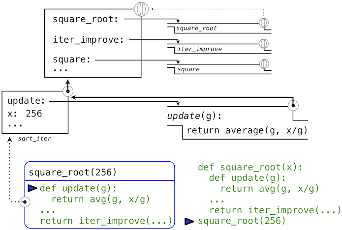
The third, pi_sum, computes the sum of terms in the series
which converges to pi very slowly.
>>> def pi_sum(n):
total, k = 0, 1
while k <= n:
total, k = total + 8 / (k * (k + 2)), k + 4
return total
>>> pi_sum(100)
3.121594652591009
These three functions clearly share a common underlying pattern. They are for the most part identical, differing
only in name, the function of k used to compute the term to be added, and the function that provides the next value
of k. We could generate each of the functions by filling in slots in the same template:
def <name>(n):
total, k = 0, 1
while k <= n:
total, k = total + <term>(k), <next>(k)
return total
26
The presence of such a common pattern is strong evidence that there is a useful abstraction waiting to be
brought to the surface. Each of these functions is a summation of terms. As program designers, we would like
our language to be powerful enough so that we can write a function that expresses the concept of summation itself
rather than only functions that compute particular sums. We can do so readily in Python by taking the common
template shown above and transforming the “slots” into formal parameters:
>>> def summation(n, term, next):
total, k = 0, 1
while k <= n:
total, k = total + term(k), next(k)
return total
Notice that summation takes as its arguments the upper bound n together with the functions term and
next. We can use summation just as we would any function, and it expresses summations succinctly:
>>> def cube(k):
return pow(k, 3)
>>> def successor(k):
return k + 1
>>> def sum_cubes(n):
return summation(n, cube, successor)
>>> sum_cubes(3)
36
Using an identity function that returns its argument, we can also sum integers.
>>> def identity(k):
return k
>>> def sum_naturals(n):
return summation(n, identity, successor)
>>> sum_naturals(10)
55
We can also define pi_sum piece by piece, using our summation abstraction to combine components.
>>> def pi_term(k):
denominator = k * (k + 2)
return 8 / denominator
>>> def pi_next(k):
return k + 4
>>> def pi_sum(n):
return summation(n, pi_term, pi_next)
>>> pi_sum(1e6)
3.1415906535898936
1.6.2 Functions as General Methods
We introduced user-defined functions as a mechanism for abstracting patterns of numerical operations so as to
make them independent of the particular numbers involved. With higher-order functions, we begin to see a more
powerful kind of abstraction: some functions express general methods of computation, independent of the partic-
ular functions they call.
27
Despite this conceptual extension of what a function means, our environment model of how to evaluate a call
expression extends gracefully to the case of higher-order functions, without change. When a user-defined function
is applied to some arguments, the formal parameters are bound to the values of those arguments (which may be
functions) in a new local frame.
Consider the following example, which implements a general method for iterative improvement and uses it to
compute the golden ratio. An iterative improvement algorithm begins with a guess of a solution to an equation.
It repeatedly applies an update function to improve that guess, and applies a test to check whether the current
guess is “close enough” to be considered correct.
>>> def iter_improve(update, test, guess=1):
while not test(guess):
guess = update(guess)
return guess
The test function typically checks whether two functions, f and g, are near to each other for the value
guess. Testing whether f(x) is near to g(x) is again a general method of computation.
>>> def near(x, f, g):
return approx_eq(f(x), g(x))
A common way to test for approximate equality in programs is to compare the absolute value of the difference
between numbers to a small tolerance value.
>>> def approx_eq(x, y, tolerance=1e-5):
return abs(x - y) < tolerance
The golden ratio, often called phi, is a number that appears frequently in nature, art, and architecture. It can
be computed via iter_improve using the golden_update, and it converges when its successor is equal to
its square.
>>> def golden_update(guess):
return 1/guess + 1
>>> def golden_test(guess):
return near(guess, square, successor)
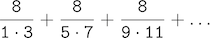
At this point, we have added several bindings to the global frame. The depictions of function values are
abbreviated for clarity.
Calling iter_improve with the arguments golden_update and golden_test will compute an ap-
proximation to the golden ratio.
>>> iter_improve(golden_update, golden_test)
1.6180371352785146
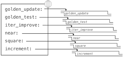
By tracing through the steps of our evaluation procedure, we can see how this result is computed. First, a
local frame for iter_improve is constructed with bindings for update, test, and guess. In the body of
iter_improve, the name test is bound to golden_test, which is called on the initial value of guess.
28
In turn, golden_test calls near, creating a third local frame that binds the formal parameters f and g to
square and successor.
Completing the evaluation of near, we see that the golden_test is False because 1 is not close to 2.
Hence, evaluation proceeds with the suite of the while clause, and this mechanical process repeats several times.
This extended example illustrates two related big ideas in computer science. First, naming and functions allow
us to abstract away a vast amount of complexity. While each function definition has been trivial, the computational
process set in motion by our evaluation procedure appears quite intricate, and we didn’t even illustrate the whole
thing. Second, it is only by virtue of the fact that we have an extremely general evaluation procedure that small
components can be composed into complex processes. Understanding that procedure allows us to validate and
inspect the process we have created.
As always, our new general method iter_improve needs a test to check its correctness. The golden ratio
can provide such a test, because it also has an exact closed-form solution, which we can compare to this iterative
result.
>>> phi = 1/2 + pow(5, 1/2)/2
>>> def near_test():
assert near(phi, square, successor), ’phi * phi is not near phi + 1’
>>> def iter_improve_test():
approx_phi = iter_improve(golden_update, golden_test)
assert approx_eq(phi, approx_phi), ’phi differs from its approximation’
New environment Feature: Higher-order functions.
Extra for experts. We left out a step in the justification of our test. For what range of tolerance values e can
you prove that if near(x, square, successor) is true with tolerance value e, then approx_eq(phi,
x) is true with the same tolerance?
1.6.3 Defining Functions III: Nested Definitions
The above examples demonstrate how the ability to pass functions as arguments significantly enhances the expres-
sive power of our programming language. Each general concept or equation maps onto its own short function.
One negative consequence of this approach to programming is that the global frame becomes cluttered with names
of small functions. Another problem is that we are constrained by particular function signatures: the update ar-
gument to iter_improve must take exactly one argument. In Python, nested function definitions address both
of these problems, but require us to amend our environment model slightly.
Let’s consider a new problem: computing the square root of a number. Repeated application of the following
update converges to the square root of x:
29
>>> def average(x, y):
return (x + y)/2
>>> def sqrt_update(guess, x):
return average(guess, x/guess)
This two-argument update function is incompatible with iter_improve, and it just provides an intermediate
value; we really only care about taking square roots in the end. The solution to both of these issues is to place
function definitions inside the body of other definitions.
>>> def square_root(x):
def update(guess):
return average(guess, x/guess)
def test(guess):
return approx_eq(square(guess), x)
return iter_improve(update, test)
Like local assignment, local def statements only affect the current local frame. These functions are only
in scope while square_root is being evaluated. Consistent with our evaluation procedure, these local def
statements don’t even get evaluated until square_root is called.
Lexical scope. Locally defined functions also have access to the name bindings in the scope in which they
are defined. In this example, update refers to the name x, which is a formal parameter of its enclosing function
square_root. This discipline of sharing names among nested definitions is called lexical scoping. Critically,
the inner functions have access to the names in the environment where they are defined (not where they are called).
We require two extensions to our environment model to enable lexical scoping.
1. Each user-defined function has an associated environment: the environment in which it was defined.
2. When a user-defined function is called, its local frame extends the environment associated with the
function.
Previous to square_root, all functions were defined in the global environment, and so they were all associ-
ated with the global environment. When we evaluate the first two clauses of square_root, we create functions
that are associated with a local environment. In the call
>>> square_root(256)
16.00000000000039
the environment first adds a local frame for square_root and evaluates the def statements for update
and test (only update is shown).
30
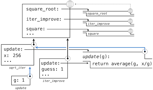
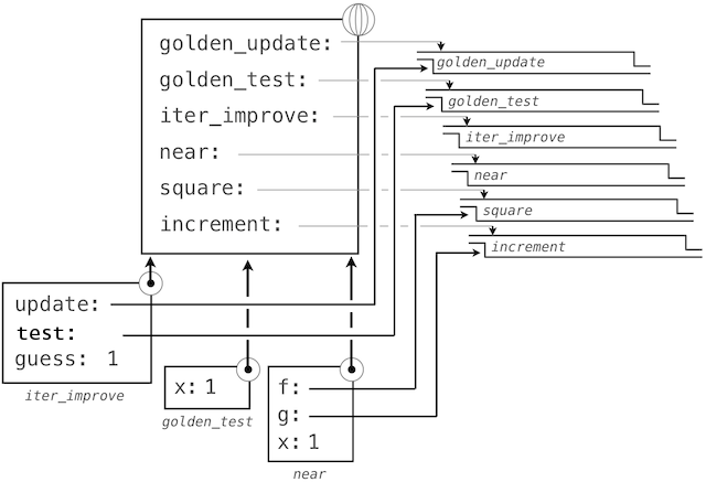
Subsequently, the name update resolves to this newly defined function, which is passed as an argument
to iter_improve. Within the body of iter_improve, we must apply our update function to the initial
guess of 1. This final application creates an environment for update that begins with a local frame containing
only g, but with the preceding frame for square_root still containing a binding for x.
The most crucial part of this evaluation procedure is the transfer of an environment associated with a function
to the local frame in which that function is evaluated. This transfer is highlighted by the blue arrows in this
diagram.
In this way, the body of update can resolve a value for x. Hence, we realize two key advantages of lexical
scoping in Python.
• The names of a local function do not interfere with names external to the function in which it is defined,
because the local function name will be bound in the current local environment in which it is defined, rather
than the global environment.
• A local function can access the environment of the enclosing function. This is because the body of the local
function is evaluated in an environment that extends the evaluation environment in which it is defined.
The update function carries with it some data: the values referenced in the environment in which it was
defined. Because they enclose information in this way, locally defined functions are often called closures.
New environment Feature: Local function definition.
1.6.4 Functions as Returned Values
We can achieve even more expressive power in our programs by creating functions whose returned values are
themselves functions. An important feature of lexically scoped programming languages is that locally defined
functions keep their associated environment when they are returned. The following example illustrates the utility
of this feature.
With many simple functions defined, function composition is a natural method of combination to include in
our programming language. That is, given two functions f(x) and g(x), we might want to define h(x) =
f(g(x)). We can define function composition using our existing tools:
>>> def compose1(f, g):
def h(x):
return f(g(x))
return h
>>> add_one_and_square = compose1(square, successor)
>>> add_one_and_square(12)
169
31
The 1 in compose1 indicates that the composed functions and returned result all take 1 argument. This
naming convention isn’t enforced by the interpreter; the 1 is just part of the function name.
At this point, we begin to observe the benefits of our investment in a rich model of computation. No modifica-
tions to our environment model are required to support our ability to return functions in this way.
1.6.5 Lambda Expressions
So far, every time we want to define a new function, we need to give it a name. But for other types of expressions,
we don’t need to associate intermediate products with a name. That is, we can compute a*b + c*d without
having to name the subexpressions a*b or c*d, or the full expression. In Python, we can create