3D graphics programming
2.1 Learning 3D graphics programming
2.2 Projecting from 3D world coordinates to 2D screen coordinates
2.4 Putting it together—MyJava3D
3D graphics programming is a fairly complex topic, worthy of a book unto itself (and there are many), but this introduction should serve as a good roadmap for further reading and give an appreciation for what Java 3D and your OpenGL or DirectX drivers are doing behind the scenes. In this chapter, I describe some of the fundamental underlying graphics techniques that allow a computer to transform a 3D scene description into a rendered image.
I’ll explain much of the needed terminology; however, if you need more information, I recommend the online 3D graphics glossaries from Mondo Media (http://www.mondomed.com/mlabs/glossary.html) , 3Dgaming.com (http://www.3dgaming.com/fps/techshop/glossary/) , and Chalmers Medialab (http://oss.medialab.chalmers.se/dictionary/).
2.1 Learning 3D graphics programming
Given the enormous variety of teaching and learning styles, there probably is no best way of teaching 3D graphics programming. I learned 3D graphics programming by experimenting. I wrote my first 3D graphics program about 10 years ago. It was written in C and ran on my venerable Intel 80386 with a whole 256 KB of RAM! Needless to say, it didn’t use Java 3D or OpenGL. The program was a modified port of a simple BASIC program that I "borrowed" from a simple little BASIC programming book. I later ported the program to run on Solaris using the GKS rendering API. The program was a very simple wire frame 3D model viewer and editor. You could load 3D shapes described using ASCII text files and then display them on screen. You could also interactively rotate the shapes about one axis. Times have certainly changed.
The interesting thing about my first 3D effort is that I built upon my general programming knowledge and some simple 2D rendering techniques, such as drawing a line to the screen. That’s what we’ll do here. In this chapter, we will turn the clock back 10 years and build some sections of that program all over again, this time using Java, Java 2D, and some of the Java 3D utilities. This should remove some of the mystery from the operations performed by 3D graphics libraries like Java 3D and OpenGL. At the end of the day, we are simply converting from 3D coordinates to 2D coordinates and drawing a bunch of points and lines. We can use the source code as a basis for introducing the basics of 3D graphics programming and highlight some of the fundamental operations that a graphics library such as Java 3D provides.
By looking at the example, you’ll see the additional operations that a real graphics API provides, and that our homegrown, primitive API does not.
To begin, look at the output from a simple Java 3D program and compare it with the test-bed application
MyJava3D. Figure 2.1 was rendered by a simple Java 3D program (the LoaderTest example), which loads a Lightwave OBJ file and renders it to the screen. Figure 2.2 was rendered in MyJava3D using AWT 2D graphics routines to draw the lines that compose the shape.
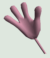
Figure 2.1 Output of a simple Java 3D application (LoaderTest)
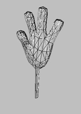
Figure 2.2 Output rendered by MyJava3D—a wire frame version of the same hand used for figure 2.1
The Java3D-rendered image is certainly superior. I’ll compare the two images in detail later in this chapter. However, the wire frame version (just lines) that was rendered using MyJava3D is also useful.
Note how the triangular surfaces that compose the 3D model are visible in figure 2.2. The model is composed of hundreds of points, each positioned in 3D space. In addition, lines are drawn to connect the points, to form triangular surfaces. The illusion of a solid 3D shape in figure 2.1 has now been revealed—what appeared to be a solid shape is in fact a hollow skin. The skin of the shape is described using hundred of points, which are then drawn as solid triangles. Java 3D filled the interior of the triangles while MyJava3D merely drew the outer lines of each triangle.
Consider the simplest series of operations that must take place to convert the 3D model data into a rendered image:
1. Load the 3D points that compose the vertices (corners) of each triangle. The vertices are indexed so they can be referenced by index later.
2. Load the connectivity information for the triangles. For example, a triangle might connect vertices 2, 5, and 7. The actual vertex information will be referenced using the information and indices established in step 1.
3. Perform some sort of mathematical conversion between the 3D coordinates for each vertex and the 2D coordinates used for the pixels on the screen. This conversion should take into account the position of the viewer of the scene as well as perspective.
4. Draw each triangle in turn using a 2D graphics context, but instead of using the 3D coordinates loaded in step 1, use the 2D coordinates that were calculated in step 3.
5. Display the image.
That’s it.
Steps 1, 2, 4, and 5 should be straightforward. Steps 1 and 2 involve some relatively simple file I/O, while steps 4 and 5 use Java’s AWT 2D graphics functions to draw a simple line into the screen. Step 3 is where much of the work takes place that qualifies this as a 3D application.
In fact, in the MyJava3D example application, we cheat and use some of the Java 3D data structures. This allows us to use the existing Lightwave OBJ loader provided with Java 3D to avoid doing the tiresome file I/O ourselves. It also provides useful data structures for describing 3D points, objects to be rendered, and so on.
2.2 Projecting from 3D world coordinates to 2D screen coordinates
Performing a simple projection from 3D coordinates to 2D coordinates is relatively uncomplicated, though it does involve some matrix algebra that I shan’t explain in detail. (There are plenty of graphics textbooks that will step you through them in far greater detail than I could here.)
There are also many introductory 3D graphics courses that cover this material online. A list of good links to frequently asked questions (FAQs) and other information is available from 3D Ark at http://www.3dark.com/resources/faqs.html. If you would like to pick up a free online book that discusses matrix and vector algebra related to 3D graphics, try Sbastien Loisel’s Zed3D, A compact reference for 3D computer graphics programming. It is available as a ZIP archive from http://www.math.mcgill.ca/~loisel/.
If you have some money to spend, I would recommend picking up the bible for these sorts of topics: Computer Graphics Principles and Practice, by James Foley, Andries van Dam, Steven Feiner, and John Hughes (Addison-Wesley, 1990).
2.2.1 A simple 3D projection routine
Here is my simple 3D-projection routine. The projectPoint method takes two Point3d instances, the first is the input 3D-coordinate while the second will be used to store the result of the projection from 3D to 2D coordinates (the z attribute will be 0). Point3d is one of the classes defined by Java 3D. Refer to the Java 3D JavaDoc for details. Essentially, it has three public members, x, y, and z that store the coordinates in the three axes.
From AwtRenderingEngine.java
private int xScreenCenter = 320/2;
private int yScreenCenter = 240/2;
private Vector3d screenPosition = new Vector3d( 0, 0, 20 );
private Vector3d viewAngle = new Vector3d( 0, 90, 180 );
private static final double DEG_TO_RAD = 0.017453292;
private double modelScale = 10;
CT = Math.cos( DEG_TO_RAD * viewAngle.x );
ST = Math.sin( DEG_TO_RAD * viewAngle.x );
CP = Math.cos( DEG_TO_RAD * viewAngle.y );
SP = Math.sin( DEG_TO_RAD * viewAngle.y );
public void projectPoint( Point3d input, Point3d output )
{
double x = screenPosition.x + input.x * CT - input.y * ST;
double y = screenPosition.y + input.x * ST * SP + input.y * CT * SP
+ input.z * CP;
double temp = viewAngle.z / (screenPosition.z + input.x * ST * CP
+ input.y * CT * CP - input.z * SP );
output.x = xScreenCenter + modelScale * temp * x;
output.y = yScreenCenter - modelScale * temp * y;
output.z = 0;
}
Let’s quickly project some points using this routine to see if it makes sense. The result of running seven 3D points through the projectPoint method is listed in table 2.1.
CT: 1
ST: 0
SP: 1
CP: 0
Table 2.1 Sample output from the projectPoint method to project points from 3D-world coordinates to 2D-screen coordinates
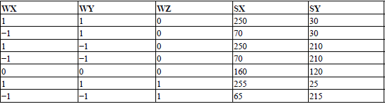
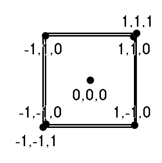
Figure 2.3 The positions of some projected points
Plotting these points by hand using a 2D graphics program (figure 2.3), you can see that they seem to make sense. Projecting the point 0,0,0 places a point at the center of the screen (160,120). While you have symmetry about the corners of the cube, increasing the Z-coordinate appears to move the two opposing corners (1,1,1 and -1,-1,1) closer to the viewer.
Taking a look at the projectPoint function again, you can see it uses the following parameters:
This very simple projection function is adequate for simple 3D projection. As you become more familiar with Java 3D, you will see that it includes far more powerful projection abilities. These allow you to render to stereo displays (such as head-mounted displays) or perform parallel projections. (In parallel projections, parallel lines remain parallel after projection.)
2.2.2 Comparing output
Look at the outputs from MyJava3D and Java 3D again (figure 2.4). They are very different—so Java 3D must be doing a lot more than projecting points and drawing lines:
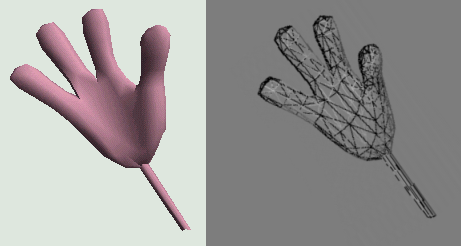
Figure 2.4 Compare the output from Java 3D (left) with the output from MyJava3D (right)
2.2.3 Drawing filled triangles
Java 3D rendered the hand as an apparently solid object. We cannot see the triangles that compose the hand, and triangles closer to the viewer obscure the triangles further away.
You could implement similar functionality within MyJava3D in several ways:
Hidden surface removal
You could calculate which triangles are not visible and exclude them from rendering. This is typically performed by enforcing a winding order on the vertices that compose a triangle. Usually vertices are connected in a clockwise order. This allows the graphics engine to calculate a vector that is normal (perpendicular) to the face of the triangle. The triangle will not be displayed if its normal vector is pointing away from the viewer.
This technique operates in object space—as it involves mathematical operations on the objects, faces, and 2 edges of the 3D objects in the scene. It typically has a computational complexity of order n2 where n is the number of faces.
This quickly becomes complicated however as some triangles may be partially visible. For partially visible triangles, an input triangle has to be broken down into several new wholly visible triangles. There are many good online graphics courses that explain various hidden-surface removal algorithms in detail. Use your favorite search engine and search on “hidden surface removal” and you will find lots of useful references.
Depth sorting (Painter’s algorithm)
The so-called Painter’s algorithm also operates in object space; however, it takes a slightly different approach. The University of North Carolina at Chapel Hill Computer Science Department online course Introduction to Computer Graphics (http://www.cs.unc.edu/~davemc/Class/136/) explains the Painter’s algorithm (http://www.cs.unc.edu/~davemc/Class/136/Lecture19/Painter.html).
The basic approach for the Painter’s algorithm is to sort the triangles in the scene by their distance from the viewer. The triangles are then rendered in order: triangle furthest away rendered first, closest triangle rendered last. This ensures that the closer triangles will overlap and obscure triangles that are further away.
An uncomplicated depth sort is easy to implement; however, once you start using it you will begin to see strange rendering artifacts. The essential problem comes down to how you measure the distance a triangle is from the viewer. Perhaps you would
With either of these simple techniques, you can generate scenes with configurations of triangles that render incorrectly. Typically, problems occur when:
For example, figure 2.5 shows some complex configurations of triangles that cannot be depth sorted using a simple algorithm.
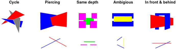
Figure 2.5 Interesting configurations of triangles that are challenging for depth-sorting algorithms
The depth of an object in the scene can be calculated if the position of the object is known and the position of the viewer or image plane is known. It would be computationally intensive to have to re-sort all the triangles in the scene every time an object or the viewer’s position changed. Fortunately, binary space partition (BSP) trees can be used to store the relative positions of the object in the scene such that they do not need to be re-sorted when the viewpoint changes. BSP trees can also help with some of the complex sorting configurations shown earlier.
Depth buffer (Z-buffer)
In contrast to the other two algorithms, the Z-buffer technique operates in image space. This is conceptually the simplest technique and is most commonly implemented within the hardware of 3D graphics cards.
If you were rendering at 640 × 480 resolution, you would also allocate a multidimensional array of integers of size 640 × 480. The array (called the depth buffer or Z-buffer) stores the depth of the closest pixel rendered into the image.
As you render each triangle in your scene, you will be drawing pixels into the frame-buffer. Each pixel has a color, and an xy-coordinate in image space. You would also calculate the z-coordinate for the pixel and update the Z-buffer. The values in the Z-buffer are the distance of each pixel in the frame from the viewer.
Before actually rendering a pixel into the frame-buffer for the screen display, inspect the Z-buffer and notice whether a pixel had already been rendered at the location that was closer to the viewer than the current pixel. If the value in the Z-buffer is less than the current pixel’s distance from the viewer, the pixel should be obscured by the closer pixel and you can skip drawing it into the frame-buffer.
It should be clear that this algorithm is fairly easy to implement, as long as you are rendering at pixel level; and if you can calculate the distance of a pixel from the viewer, things are pretty straightforward. This algorithm also has other desirable qualities: it can cope with complex intersecting shapes and it doesn’t need to split triangles. The depth testing is performed at the pixel level, and is essentially a filter that prevents some pixel rendering operations from taking place, as they have already been obscured.
The computational complexity of the algorithm is also far more manageable and it scales much better with large numbers of objects in the scene. To its detriment, the algorithm is very memory hungry: when rendering at 1024 × 800 and using 32-bit values for each Z-buffer entry, the amount of memory required is 6.25 MB.
The memory requirement is becoming less problematic, however, with newer video cards (such as the nVidia Geforce II/III) shipping with 64 MB of memory.
The Z-buffer is susceptible to problems associated with loss of precision. This is a fairly complex topic, but essentially there is a finite precision to the Z-buffer. Many video cards also use 16-bit Z-buffer entries to conserve memory on the video card, further exacerbating the problem. A 16-bit value can represent 65,536 values—so essentially there are 65,536 depth buckets into which each pixel may be placed. Now imagine a scene where the closest object is 2 meters away and the furthest object is 100,000 meters away. Suddenly only having 65,536 depth values does not seem so attractive. Some pixels that are really at different distances are going to be placed into the same bucket. The precision of the Z-buffer then starts to become a problem and entries that should have been obscured could become randomly rendered. Thirty-two-bit Z-buffer entries will obviously help matters (4,294,967,296 entries), but greater precision merely shifts the problem out a little further. In addition, precision within the Z-buffer is not uniform as described here; there is greater precision toward the front of the scene and less precision toward the rear.
When rendering using a Z-buffer, the rendering system typically requires that you specify a near and a far clipping plane. If the near clipping plane is located at z = 2 and the far plane is located at z = 10, then only objects that are between 2 and 10 meters from the viewer will get rendered. A 16-bit Z-buffer would then be quantized into 65,536 values placed between 2 and 10 meters. This would give you very high precision and would be fine for most applications. If the far plane were moved out to z = 50,000 meters then you will start to run into precision problems, particularly at the back of the visible region.
In general, the ratio between the far and near clipping (far/near) planes should be kept to below 1,000 to avoid loss of precision. You can read a detailed description of the precision issues with the OpenGL depth buffer at the OpenGL FAQ and Troubleshooting Guide (http://www.frii.com/~martz/oglfaq/depthbuffer.htm).
MyJava3D includes some simple lighting calculations. The lighting equation sets the color of a line to be proportional to the angle between the surface and the light in the scene. The closer a surface is to being perpendicular to the vector representing a light ray, the brighter the surface should appear. Surfaces that are perpendicular to light rays will absorb light and appear brighter. MyJava3D includes a single white light and uses the Phong lighting equation to calculate the intensity for each triangle in the model (figure 2.6).
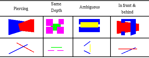
Figure 2.6 MyJava3D rendering without light intensity calculations
The computeIntensity method calculates the color intensity to use when rendering a triangle. It accepts a GeometryArray containing the 3D points for the geometry, an index that is the first point to be rendered, and a count of the number of points (vertices) that compose the item to be rendered.
The method then computes the average normal vector for the points to be rendered by inspecting the normal vectors stored within the GeometryArray. For a triangle (three vertices) this will be the vector normal to the plane of the surface.
The angle between the surface normal and the viewer is then calculated (beta). If the cosine of this angle is less than or equal to zero, the facet cannot be seen by the viewer and an intensity of zero will be returned. Otherwise, the method computes the angle between the light source position vector and the surface normal vector of the surface (theta). If the cosine of this angle is less than or equal to zero, none of the light from the light source illuminates the surface, so its light intensity is set to that of the ambient light. Otherwise, the surface normal vector is multiplied by the cosine of theta, the resulting vector is normalized, and then the light vector subtracted from it and the resulting vector normalized again. The angle between this vector and the viewer vector (alpha) is then determined. The intensity of the surface is the sum of the ambient light, the diffuse lighting from the surface multiplied by the cosine of the theta, and the specular light from the surface multiplied by the cosine of alpha raised to the glossiness power. The last term is the Phong shading, which creates the highlights that are seen in illuminated curved objects.
Note that in this simple MyJava3D example only one light is being used to illuminate the scene—in Java3D, OpenGL, or Direct3D many lights can be positioned within the scene and the rendering engine will compute the combined effects of all the lights on every surface.
Please refer to chapter 10 for a further discussion of lighting equations and example illustrations created using Java 3D.
From AwtRenderingEngine.java
private int computeIntensity( GeometryArray geometryArray, int index, int numPoints )
{
int intensity = 0;
if ( computeIntensity != false )
{
// if we have a normal vector, compute the intensity
// under the lighting
if ( (geometryArray.getVertexFormat( ) GeometryArray.NORMALS) == GeometryArray.NORMALS )
{
double cos_theta;
double cos_alpha;
double cos_beta;
for( int n = 0; n <numPoints; n++ )
geometryArray.getNormal( index+n, normalsArray[n] );
// take the average normal vector
averageVector( surf_norm, normalsArray, numPoints );
temp.set( view );
temp.scale( 1.0f, surf_norm );
cos_beta = temp.x + temp.y + temp.z;
if ( cos_beta > 0.0 )
{
cos_theta = surf_norm.dot( light );
if ( cos_theta <= 0.0 )
{
intensity = (int) (lightMax * lightAmbient);
}
else
{
temp.set( surf_norm );
temp.scale( (float) cos_theta );
temp.normalize( );
temp.sub( light );
temp.normalize( );
cos_alpha = view.dot( temp );
intensity = (int) (lightMax * ( lightAmbient +
lightDiffuse * cos_theta + lightSpecular *
Math.pow( cos_alpha, lightGlossiness )));
}
}
}
}
return intensity;
}
_________________________________________________________________
2.4 Putting it together—MyJava3D
The MyJava3D example defines the RenderingEngine interface. This interface defines a simple rendering contract between a client and a 3D renderer implementation. The RenderingEngine interface defines a simple renderer that can render 3D geometry described using a Java 3D GeometryArray. The GeometryArray contains the 3D points and normal vectors for the 3D model to be rendered.
In addition to adding GeometryArrays to the RenderingEngine (addGeometry method), the viewpoint of the viewer can be specified (setViewAngle), the direction of a single light can be specified (setLightAngle), the scaling factor to be applied to the model can be varied (setScale), and the size of the rendering screen defined (setScreenSize).
To render all the GeometryArrays added to the RenderingEngine using the current light, screen, scale, and view parameters, clients can call the render method, supplying a Graphics object to render into, along with an optional GeometryUpdater. The GeometryUpdater allows a client to modify the positions of points or rendering parameters prior to rendering.
From AwtRenderingEngine.java
/**
* Definition of the RenderingEngine interface. A RenderingEngine
* can render 3D geometry (described using a Java 3D GeometryArray)
* into a 2D Graphics context.
*/
public interface RenderingEngine
{
/**
* Add a GeometryArray to the RenderingEngine. All GeometryArrays
* will be rendered.
*/
public void addGeometry( GeometryArray geometryArray );
/**
* Render a single frame into the Graphics.
*/
public void render( Graphics graphics, GeometryUpdater updater );
/**
* Get the current Screen position used by the RenderEngine.
*/
public Vector3d getScreenPosition();
/**
* Get the current View Angle used by the RenderEngine. View
* angles are expressed in degrees.
*/
public Vector3d getViewAngle();
/**