General Chemistry II by John Hutchinson - HTML preview
Download the book in PDF, ePub for a complete version.

General Chemistry II
By: John Hutchinson
Online: < http://cnx.org/content/col10262/1.2>
This selection and arrangement of content as a collection is copyrighted by John Hutchinson.
It is licensed under the Creative Commons Attribution License: http://creativecommons.org/licenses/by/1.0
Collection structure revised: 2005/03/25
For copyright and attribution information for the modules contained in this collection, see the " Attributions" section at the end of the collection.
General Chemistry II
Table of Contents
Observation 1: Pressure-Volume Measurements on Gases
Observation 2: Volume-Temperature Measurements on Gases
Observation 3: Partial Pressures
Review and Discussion Questions
Chapter 2. The Kinetic Molecular Theory
Observation 1: Limitations of the Validity of the Ideal Gas Law
Observation 2: Density and Compressibility of Gas
Postulates of the Kinetic Molecular Theory
Derivation of Boyle's Law from the Kinetic Molecular Theory
Analysis of Deviations from the Ideal Gas Law
Observation 3: Boiling Points of simple hydrides
Review and Discussion Questions
Chapter 3. Phase Equilibrium and Intermolecular Interactions
Observation 1: Gas-Liquid Phase Transitions
Observation 2: Vapor pressure of a liquid
Observation 4: Dynamic Equilibrium
Review and Discussion Questions
Chapter 4. Reaction Equilibrium in the Gas Phase
Observation 1: Reaction equilibrium
Observation 2: Equilibrium constants
Observation 3: Temperature Dependence of the Reaction Equilibrium
Observation 4: Changes in Equilibrium and Le Châtelier's Principle
Review and Discussion Questions
Chapter 5. Acid-Base Equilibrium
Observation 1: Strong Acids and Weak Acids
Observation 2: Percent Ionization in Weak Acids
Observation 3: Autoionization of Water
Observation 4: Base Ionization, Neutralization and Hydrolysis of Salts
Observation 5: Acid strength and molecular properties
Review and Discussion Questions
Observation 2: Rate Laws and the Order of Reaction
Concentrations as a Function of Time and the Reaction Half-life
Observation 3: Temperature Dependence of Reaction Rates
Collision Model for Reaction Rates
Observation 4: Rate Laws for More Complicated Reaction Processes
Review and Discussion Questions
Chapter 7. Equilibrium and the Second Law of Thermodynamics
Observation 1: Spontaneous Mixing
Observation 2: Absolute Entropies
Observation 3: Condensation and Freezing
Thermodynamic Description of Phase Equilibrium
Thermodynamic description of reaction equilibrium
Thermodynamic Description of the Equilibrium Constant
Review and Discussion Questions

Chapter 1. The Ideal Gas Law
Foundation
We assume as our starting point the atomic molecular theory. That is, we assume that all matter is
composed of discrete particles. The elements consist of identical atoms, and compounds consist of
identical molecules, which are particles containing small whole number ratios of atoms. We also
assume that we have determined a complete set of relative atomic weights, allowing us to
determine the molecular formula for any compound.
Goals
The individual molecules of different compounds have characteristic properties, such as mass,
structure, geometry, bond lengths, bond angles, polarity, diamagnetism or paramagnetism. We
have not yet considered the properties of mass quantities of matter, such as density, phase (solid,
liquid or gas) at room temperature, boiling and melting points, reactivity, and so forth. These are
properties which are not exhibited by individual molecules. It makes no sense to ask what the
boiling point of one molecule is, nor does an individual molecule exist as a gas, solid, or liquid.
However, we do expect that these material or bulk properties are related to the properties of the
individual molecules. Our ultimate goal is to relate the properties of the atoms and molecules to
the properties of the materials which they comprise.
Achieving this goal will require considerable analysis. In this Concept Development Study, we
begin at a somewhat more fundamental level, with our goal to know more about the nature of
gases, liquids and solids. We need to study the relationships between the physical properties of
materials, such as density and temperature. We begin our study by examining these properties in
gases.
Observation 1: Pressure-Volume Measurements on Gases
It is an elementary observation that air has a "spring" to it: if you squeeze a balloon, the balloon
rebounds to its original shape. As you pump air into a bicycle tire, the air pushes back against the
piston of the pump. Furthermore, this resistance of the air against the piston clearly increases as
the piston is pushed farther in. The "spring" of the air is measured as a pressure, where the
pressure P is defined
(1.1)
F is the force exerted by the air on the surface of the piston head and A is the surface area of the piston head.
For our purposes, a simple pressure gauge is sufficient. We trap a small quantity of air in a
syringe (a piston inside a cylinder) connected to the pressure gauge, and measure both the volume
of air trapped inside the syringe and the pressure reading on the gauge. In one such sample
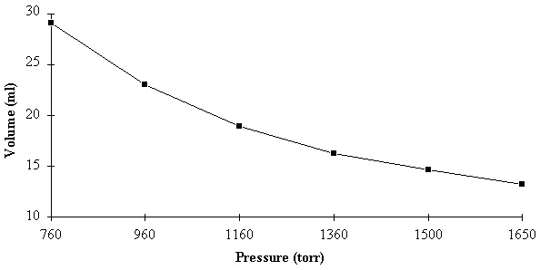
measurement, we might find that, at atmospheric pressure (760 torr), the volume of gas trapped
inside the syringe is 29.0 ml. We then compress the syringe slightly, so that the volume is now
23.0 ml. We feel the increased spring of the air, and this is registered on the gauge as an increase
in pressure to 960 torr. It is simple to make many measurements in this manner. A sample set of
data appears in Table 1.1. We note that, in agreement with our experience with gases, the pressure increases as the volume decreases. These data are plotted here.
Table 1.1. Sample Data from
Pressure-Volume Measurement
Pressure (torr) Volume (ml)
760
29.0
960
23.0
1160
19.0
1360
16.2
1500
14.7
1650
13.3
Figure 1.1. Measurements on Spring of the Air
An initial question is whether there is a quantitative relationship between the pressure
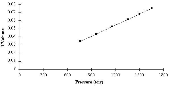


measurements and the volume measurements. To explore this possibility, we try to plot the data in
such a way that both quantities increase together. This can be accomplished by plotting the
pressure versus the inverse of the volume, rather than versus the volume. The data are given in
Table 1.2. Analysis of Sample Data
Pressure (torr) Volume (ml) 1/Volume (1/ml) Pressure × Volume
760
29.0
0.0345
22040
960
23.0
0.0435
22080
1160
19.0
0.0526
22040
1360
16.2
0.0617
22032
1500
14.7
0.0680
22050
1650
13.3
0.0752
21945
Figure 1.2. Analysis of Measurements on Spring of the Air
Notice also that, with elegant simplicity, the data points form a straight line. Furthermore, the
straight line seems to connect to the origin {0, 0}. This means that the pressure must simply be a
constant multiplied by :
(1.2)
If we multiply both sides of this equation by V, then we notice that
(1.3)
PV= k
In other words, if we go back and multiply the pressure and the volume together for each
experiment, we should get the same number each time. These results are shown in the last column
of Table 1.2, and we see that, within the error of our data, all of the data points give the same value of the product of pressure and volume. (The volume measurements are given to three
decimal places and hence are accurate to a little better than 1%. The values of
(Pressure × Volume) are all within 1% of each other, so the fluctuations are not meaningful.)
We should wonder what significance, if any, can be assigned to the number 22040( torrml) we
have observed. It is easy to demonstrate that this "constant" is not so constant. We can easily trap
any amount of air in the syringe at atmospheric pressure. This will give us any volume of air we
wish at 760 torr pressure. Hence, the value 22040( torrml) is only observed for the particular
amount of air we happened to choose in our sample measurement. Furthermore, if we heat the
syringe with a fixed amount of air, we observe that the volume increases, thus changing the value
of the 22040( torrml). Thus, we should be careful to note that the product of pressure and
volume is a constant for a given amount of air at a fixed temperature. This observation is
referred to as Boyle's Law, dating to 1662.
The data given in Table 1.1 assumed that we used air for the gas sample. (That, of course, was the only gas with which Boyle was familiar.) We now experiment with varying the composition of the
gas sample. For example, we can put oxygen, hydrogen, nitrogen, helium, argon, carbon dioxide,
water vapor, nitrogen dioxide, or methane into the cylinder. In each case we start with 29.0 ml of
gas at 760 torr and 25°C. We then vary the volumes as in Table 1.1 and measure the pressures.
Remarkably, we find that the pressure of each gas is exactly the same as every other gas at each
volume given. For example, if we press the syringe to a volume of 16.2 ml, we observe a pressure
of 1360 torr, no matter which gas is in the cylinder. This result also applies equally well to
mixtures of different gases, the most familiar example being air, of course.
We conclude that the pressure of a gas sample depends on the volume of the gas and the
temperature, but not on the composition of the gas sample. We now add to this result a conclusion
from a previous study. Specifically, we recall the Law of Combining Volumes, which states that, when gases combine during a chemical reaction at a fixed pressure and temperature, the ratios of
their volumes are simple whole number ratios. We further recall that this result can be explained
in the context of the atomic molecular theory by hypothesizing that equal volumes of gas contain
equal numbers of gas particles, independent of the type of gas, a conclusion we call Avogadro's
Hypothesis. Combining this result with Boyle's law reveals that the pressure of a gas depends on
the number of gas particles, the volume in which they are contained, and the temperature of the sample. The pressure does not depend on the type of gas particles in the sample or whether they
are even all the same.
We can express this result in terms of Boyle's law by noting that, in the equation PV= k, the
"constant" k is actually a function which varies with both number of gas particles in the sample and the temperature of the sample. Thus, we can more accurately write
(1.4)
PV= k( N, t)
explicitly showing that the product of pressure and volume depends on N, the number of particles
in the gas sample, and t,the temperature.
It is interesting to note that, in 1738, Bernoulli showed that the inverse relationship between
pressure and volume could be proven by assuming that a gas consists of individual particles
colliding with the walls of the container. However, this early evidence for the existence of atoms
was ignored for roughly 120 years, and the atomic molecular theory was not to be developed for
another 70 years, based on mass measurements rather than pressure measurements.
Observation 2: Volume-Temperature Measurements on Gases
We have already noted the dependence of Boyle's Law on temperature. To observe a constant
product of pressure and volume, the temperature must be held fixed. We next analyze what
happens to the gas when the temperature is allowed to vary. An interesting first problem that
might not have been expected is the question of how to measure temperature. In fact, for most
purposes, we think of temperature only in the rather non-quantitative manner of "how hot or cold"
something is, but then we measure temperature by examining the length of mercury in a tube, or
by the electrical potential across a thermocouple in an electronic thermometer. We then briefly
consider the complicated question of just what we are measuring when we measure the
temperature.
Imagine that you are given a cup of water and asked to describe it as "hot" or "cold." Even without a calibrated thermometer, the experiment is simple: you put your finger in it. Only a qualitative
question was asked, so there is no need for a quantitative measurement of "how hot" or "how
cold." The experiment is only slightly more involved if you are given two cups of water and asked
which one is hotter or colder. A simple solution is to put one finger in each cup and to directly
compare the sensation. You still don't need a calibrated thermometer or even a temperature scale
at all.
Finally, imagine that you are given a cup of water each day for a week at the same time and are
asked to determine which day's cup contained the hottest or coldest water. Since you can no longer
trust your sensory memory from day to day, you have no choice but to define a temperature scale.
To do this, we make a physical measurement on the water by bringing it into contact with
something else whose properties depend on the "hotness" of the water in some unspecified way.
(For example, the volume of mercury in a glass tube expands when placed in hot water; certain
strips of metal expand or contract when heated; some liquid crystals change color when heated;
etc. ) We assume that this property will have the same value when it is placed in contact with two
objects which have the same "hotness" or temperature. Somewhat obliquely, this defines the
temperature measurement.

For simplicity, we illustrate with a mercury-filled glass tube thermometer. We observe quite
easily that when the tube is inserted in water we consider "hot," the volume of mercury is larger
than when we insert the tube in water that we consider "cold." Therefore, the volume of mercury is
a measure of how hot something is. Furthermore, we observe that, when two very different objects
appear to have the same "hotness," they also give the same volume of mercury in the glass tube.
This allows us to make quantitative comparisons of "hotness" or temperature based on the volume
of mercury in a tube.
All that remains is to make up some numbers that define the scale for the temperature, and we can
literally do this in any way that we please. This arbitrariness is what allows us to have two
different, but perfectly acceptable, temperature scales, such as Fahrenheit and Centigrade. The
latter scale simply assigns zero to be the temperature at which water freezes at atmospheric
pressure. We then insert our mercury thermometer into freezing water, and mark the level of the
mercury as "0". Another point on our scale assigns 100 to be the boiling point of water at
atmospheric pressure. We insert our mercury thermometer into boiling water and mark the level
of mercury as "100." Finally, we just mark off in increments of
of the distance between the "0"
and the "100" marks, and we have a working thermometer. Given the arbitrariness of this way of
measuring temperature, it would be remarkable to find a quantitative relationship between
temperature and any other physical property.
Yet that is what we now observe. We take the same syringe used in the previous section and trap
in it a small sample of air at room temperature and atmospheric pressure. (From our observations
above, it should be clear that the type of gas we use is irrelevant.) The experiment consists of
measuring the volume of the gas sample in the syringe as we vary the temperature of the gas
sample. In each measurement, the pressure of the gas is held fixed by allowing the piston in the
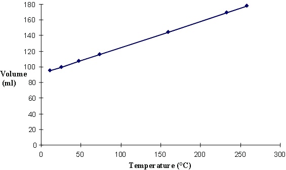
syringe to move freely against atmospheric pressure. A sample set of data is shown in Table 1.3
and plotted here.
Table 1.3. Sample Data from
Volume-Temperature
Measurement
Temperature (°C) Volume (ml)
11
95.3
25
100.0
47
107.4
73
116.1
159
145.0


233
169.8
258
178.1
Figure 1.3. Volume vs. Temperature of a Gas
We find that there is a simple linear (straight line) relationship between the volume of a gas and
its temperature as measured by a mercury thermometer. We can express this in the form of an
equation for a line:
(1.5)
V= αt+ β
where V is the volume and t is the temperature in °C. α and β are the slope and intercept of the line, and in this case, α=0.335 and, β=91.7. We can rewrite this equation in a slightly different form:
(1.6)
This is the same equation, except that it reveals that the quantity must be a temperature, since
we can add it to a temperature. This is a particularly important quantity: if we were to set the
temperature of the gas equal to
, we would find that the volume of the gas would be
exactly 0! (This assumes that this equation can be extrapolated to that temperature. This is quite
an optimistic extrapolation, since we haven't made any measurements near to -273°C. In fact, our
gas sample would condense to a liquid or solid before we ever reached that low temperature.)
Since the volume depends on the pressure and the amount of gas (Boyle's Law), then the values of
α and β also depend on the pressure and amount of gas and carry no particular significance.
However, when we repeat our observations for many values of the amount of gas and the fixed


pressure, we find that the ratio
does not vary from one sample to the next. Although we
do not know the physical significance of this temperature at this point, we can assert that it is a
true constant, independent of any choice of the conditions of the experiment. We refer to this
temperature as absolute zero, since a temperature below this value would be predicted to produce
a negative gas volume. Evidently, then, we cannot expect to lower the temperature of any gas
below this temperature.
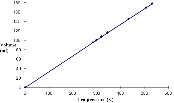
This provides us an "absolute temperature scale" with a zero which is not arbitrarily defined. This
we define by adding 273 (the value of ) to temperatures measured in °C, and we define this scale
to be in units of degrees Kelvin (K). The data in Table 1.3 are now recalibrated to the absolute temperature scale in Table 1.4 and plotted here.
Table 1.4. Analysis of Volume-Temperature Data
Temperature (°C) Temperature (K) Volume (ml)
11
284