1 Basics & Beyond......................................................................................................... 4
1.1 Introduction......................................................................................................... 4 1.2 The EXCEL Screen............................................................................................. 4
1.3 Moving Around................................................................................................... 5 2 Data Entry ................................................................................................................... 8
2.1 Text ..................................................................................................................... 8 2.2 Number (including date, time, percent) .............................................................. 8
2.3 Formulae ............................................................................................................. 8 2.4 Functions............................................................................................................. 9 2.5 AutoComplete ..................................................................................................... 9 2.6 AutoCorrect....................................................................................................... 10 2.7 AutoFill ............................................................................................................. 10 2.8 Data Validation ................................................................................................. 11 3 Totals & More........................................................................................................... 13 3.1 + + + ,…. why not? ........................................................................................... 13
3.2 SUM() Function ................................................................................................ 13 3.3 QuickSum ......................................................................................................... 13 3.4 SUBTOTAL() Function.................................................................................... 14 3.5 SUMIF() Function ............................................................................................ 14 3.6 Sorting Data ...................................................................................................... 14 3.7 Sub-Totals ......................................................................................................... 15 3.8 Conditional Sum Add-In................................................................................... 16 4 Queries in Lists ......................................................................................................... 17
4.1 AutoFilter.......................................................................................................... 17 4.2 Advanced Filter................................................................................................. 17 5 Functions................................................................................................................... 19
5.1 Lookup Functions ............................................................................................. 19 5.2 Date Functions .................................................................................................. 19 5.3 Numeric Functions............................................................................................ 21 5.4 Text Functions .................................................................................................. 21 5.5 Financial Functions........................................................................................... 21 5.6 Some more functions ........................................................................................ 22 6 The Look & Feel of Output ...................................................................................... 24
6.1 Formatting......................................................................................................... 24 6.2 Styles................................................................................................................. 25 6.3 Conditional Formatting..................................................................................... 26 6.4 Custom Views................................................................................................... 26 6.5 Printing.............................................................................................................. 27 6.6 Saying it with Charts......................................................................................... 27
7 Copying & Moving ................................................................................................... 28 7.1 Paste Special ..................................................................................................... 29 8 Saving Work & Protecting It .................................................................................... 30
8.1 File-Level Protection ........................................................................................ 30 9 Analysing Data.......................................................................................................... 32 9.1 Data Tables ....................................................................................................... 32 9.2 Scenarios ........................................................................................................... 33 9.3 Goal Seek .......................................................................................................... 33 9.4 Solver ................................................................................................................ 33 10 PivotTables ........................................................................................................... 35 10.1 Creating a Pivot Table ...................................................................................... 35
10.2 Layout of the PivotTable .................................................................................. 37
10.3 Some Examples:................................................................................................ 37 11 Auditing Tools ...................................................................................................... 41 11.1 Auditing Toolbar............................................................................................... 41 11.2 Documenting a Sheet ........................................................................................ 41
11.3 Migrating Data from Other Software................................................................ 43
11.4 Common Audit Techniques .............................................................................. 43
12 Automating MS-EXCEL ...................................................................................... 44 12.1 Open EXCEL each time computer starts .......................................................... 44
12.2 Open a particular file each time EXCEL starts................................................. 44
12.3 Create a new file based on a template each time computer starts..................... 44
12.4 Specifying the Defaults in EXCEL................................................................... 44
12.5 Customizing Menus & Toolbars....................................................................... 45
12.6 Customization Options...................................................................................... 46 12.7 Templates.......................................................................................................... 46 12.8 Workspaces.. ..................................................................................................... 47 12.9 Talking with Other Software ............................................................................ 47
13 Introduction to Macros.......................................................................................... 48
13.1 Global Macros vs. Individual Macros............................................................... 48
13.2 Use of Macro Recorder..................................................................................... 49
13.3 Running Macros................................................................................................ 49 13.4 Basics of VB Programming .............................................................................. 51
1 ANNEXURE A: KEYBOARD SHORTCUTS ........................................................ 53
2 ANNEXURE “B” IMPORTANT EXCEL FUNCTIONS........................................ 55
3 ANNEXURE “C”: COMMON ERROR CODES .................................................... 59
4 ANNEXURE “D” LIST OF ADD-INS PROVIDED WITH MS-EXCEL .............. 61
Microsoft Excel is a spreadsheet program that is designed to record and analyze numbers and data. Excel is very widely used for accounting and financial purposes.
The files created in Excel are known as workbooks. In turn, each workbook can contain one or more worksheets. An Excel worksheet is laid out like a grid with horizontal rows and vertical columns. Columns are labeled with alphabets (A, B, C, etc.) while rows are given numbers (1, 2, 3, etc.). The intersection of a row and a column is called a cell. A cell is referred by a combination of column alphabet and row number (A1, A2, etc.). A cell is a primary unit of measure in Excel and all the information is stored in cells. . A range is a collection of contiguous cells (which form a rectangular block) on which the user wants to perform similar type of calculations. A range is referred to by a combination of the cell addresses of the diagonally opposite cells separated by a colon (A1:D6)
1.2 The EXCEL ScreenOn loading MS-EXCEL (either through the shortcut menu, or icon on desktop or through the Start Menu), the following screen appears:

The various components of the EXCEL Screen are explained in brief below: Sr. Contains Remarks
1 Title Bar
3 Tool Bars
4 Formula Bar
5 Column Labels
6 Row Labels
7 Sheet Area
8 Sheet Tab Contains the name of the File currently open and also has the window control buttons to either close or minimize the program0
Contains the list of various commands that can be performed in MS-EXCEL. It can be invoked either by a mouse click or the Alt Key from the keyboard
Contain buttons for some commonly performed tasks. The commands can be activated by a mere mouse-click Displays the content of the active cell. The left hand side of this bar includes the name box which contains the list of all the range names and thereby facilitates quicker worksheet navigation
Contains the headings of the columns. Can be used for column-wide operations like increasing column width, hiding columns, formatting entire columns, etc.
Contains the headings of the rows. Can be used for rowwide operations like increasing row height, hiding rows, formatting entire rows, etc.
The place where the actual data is entered. The Active Cell is surrounded by a dark rectangle.
Gives reference to the sheet which is currently active. One can quickly navigate through different sheets from here
9 Additional Tool Some additional toolbars Bars
10 Status Bar
12 Application
Control Buttons Includes the various information sent by EXCEL. Of particular use is the QuickSum Feature in the status bar which automatically displays the totals of the selected cells The Scroll Bars can be used for quick movement within a worksheet. The extreme top of the vertical scroll bar and the extreme right of the horizontal scroll bar contain a split indicator which permits the user to divide the sheet into two parts.
These buttons are used to minimize or control the size of a particular file.
1.3 Moving Around
A worksheet can contain upto 65,536 rows and 256 columns whereas the visibility of the information on the screen is restricted to the size of the screen (generally 18-20 rows and 8-10 columns are visible at a time). Therefore, one may need to move around different sections of a worksheet. There are various ways in which one can move around very efficiently.
1.3.1 Keyboard Shortcuts
The most widely used option is of course a wheel-mouse but at times, the keyboard is very handy. For example, to reach the last entered cell in a worksheet one just uses the <Ctrl>+<End> combination. Similarly, <Ctrl>+<Home> takes one to the first cell of the
worksheet (which is always A1). Using <Home> takes one to the first cell of the particular row. <End> can be used with the combination of the arrow keys to reach at the end of the list in the particular direction. A complete list of keyboard shortcuts is provided in Annexure “A”
1.3.2 Range NamesSometimes it is convenient to use a descriptive name to name a cell or a range of cells. Named ranges can also be used in formulas and functions. To name a range: 1. Select the range to be named.
2. Click the Name box on the left side of the formula bar
3. Type the range name (up to 255 characters). Valid names cannot use spaces and the first character must not be a number. Also, the name cannot look like a cell address such as B14.
4. Press Enter.
OR
1. Select the range
2. Select Insert/Name
3. Choose Define
4. Type the name of the range.
1.3.3 Window Split & Freeze
Many a times, one wants to refer to two different sections of a worksheet. For example, in case of a long list, the headings might scroll up. In that event, one can consider to split the window into two parts. One can split the windows by dragging the split handle which
appears at the extreme top of the vertical scroll bar and the extreme right of the horizontal scroll bar. In the alternative, one can position the cell pointer to the cell where one desires a split and choose the command Split from the Window Menu. To remove the split, either re-drag the split bar or choose Window->Unsplit.
While the movement of the split windows is synchronized, none of them is fixed. Therefore, it is possible to loose track of the titles if the mouse movements are not properly handled. To avoid such a situation, one can choose Window->Freeze Panes. To reverse the process, choose Window->Unfreeze Panes.
1.3.4 Multiple WindowsWindows Split does not permit asynchronous viewing. For such a purpose, one can consider opening multiple windows of the same file. To do this, choose Window-> New Window. Re-size both the windows using the mouse pointer. Of course, multiple windows of the same file are at times confusing to handle.
Information entered into a cell is understood either as a text entry, a value or a formula. Functions are also treated equivalent to formulae. Dates, time and percentages are stored as numbers (values). It is important that a particular information is stored in the correct format.
2.1 TextText entries or labels can contain any combination of letters, numbers and spaces. A label which is too long for the width of a cell floats across the cells to its right / left / both (depending on the alignment of the cell) as long as those cells do not contain any information. If the cells aren’t empty, the label is truncated or cut-off. By default, labels are left-justified.
2.2 Number (including date, time, percent)Numbers and text are treated differently. The default alignment for text is left whereas for numbers, it is right. Secondly, if a value is too large to fit in the current cell width, Excel displays a series of # characters as a error signal. A list of various error signals and what they denote is enclosed as Annexure “C”. Values are displayed in the General Number Format. This display can be customized using the Format Cells command.
2.3 FormulaeA cell can also derive the value though a formula. The building of a formula is intuitive and can be easily mastered through practice. For example, if Cell A1 contains 3000 being the tax payable and you want to calculate the surcharge, go to Cell A2 and type the formula +A1*5% (as the surcharge rate is 5%) and Excel does the calculation for you. To get the gross tax liability, go to Cell A3 and say +A1+A2 (as gross tax includes tax and surcharge). The formula can also be built by pointing to the dependent cells instead of typing the cell address. Excel evaluates a formula in a particular order of precedence. The operators used in a formula and precedence accorded by EXCEL are as under:
Operator Description Precedence : Range of Cells 1
, Union of Cells 2
% Percentage 3 ^ Exponentiation 4 * Multiplication 5 / Division 6 + Addition 7
- Subtraction 8 & Concatenation 9 = < > Comparison Operators 10
If the order of evaluation is to be changed, parenthesis should be used to group expressions within a formula. If more than one pair of parenthesis is present in a formula, Excel evaluates the expression in the innermost parenthesis first.
A cell can also derive its value through functions. Functions are processes, which have been defined and standardized by Excel. A complete list of functions can be found at Insert -> Function. A list of commonly used functions is enclosed as “Annexure B”. Few more common functions include the SUM function (which totals all the numbers in a particular range – of course, EXCEL also has the QuickSum Feature which displays the sum of the selected range in the bottom pane) and the IF function used to manage alternate calculations in varying situations (it is very simple to use and can be nested, but take care to use the brackets appropriately otherwise the results can be disastrous!). A very common example of the use of IF function is to calculate the tax payable by an individual. For example, if cell B3 contains the net taxable income of an individual, the tax payable by him (excluding surcharge) can be calculated using a nested IF function as stated: =IF(B3>150000,(+B3-150000)*0.3+19000,IF(B3>60000,(B3-60000)*0.2+1000,
2.4.1 Using the Function Builder
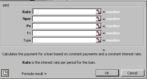
A function takes in certain standard arguments, undertakes the evaluation process and returns a particular result. In case one is unaware of the arguments, one can type the function name along with the opening parenthesis and click on the = sign on the Formula Bar. The Function Wizard presents the list of arguments and the brief description of the
arguments. In such a fashion, one can build a formula through a Wizard and simultaneously learn the function itself. For example, the Function Builder Dialog Box in the case of PMT function is shown below:
 2.5 AutoComplete
Manual data entry into a range of cells can be made faster with the assistance of AutoComplete - a feature which suggests the current cell entry based on the existing list. It should however be noted that AutoComplete has certain limitations – it does not work if there is a blank cell in the list, it works only when a unique combination consisting of at least one alphabet is met in the list. In case of multiple similar entries, a better option is the Pick from List which appears in the right-click shortcut of the mouse.
2.6 AutoCorrectThe AutoCorrect feature automatically corrects common typing errors as you type. For this purpose, Excel uses a database of commonly misspelled words. This database can be customized from the Tools -> AutoCorrect Menu. The following screen comes up:
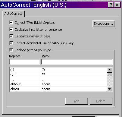
One can use the AutoCorrect feature to quickly type some normal text which is regularly used in an organization. For example, the organization name can be made a subject matter of AutoCorrect to speeden up data entry.
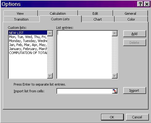
2.7 AutoFillAutoFill is an in-built feature whereby one can fill up a particular range of cells based on some pre-determined series. For example, if one cell contains January and the next one contains February, one can just use the fill handle to automatically complete the entire range with the month names. One can create custom lists pertaining to one’s organization (for example, plant locations) from Tools -> Options -> Custom Lists. The following screen appears where one can either type in the required items or pick from a range of cells
 2.8 Data Validation
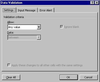
At times, there may be a need to restrict the content that is being typed into a particular cell. For example, one may want the residential status to be either “Resident” or “Resident but Not Ordinarily Resident” or “Non Resident”. In such a case, the entry into a particular cell can be validated through the “Data Validation” Feature. The steps for data validation feature are explained below:
1. Select the cell/range for which validation is to be applied2. Choose Data -> Validation from the menu. The following screen appears
3. This feature validates only Keyboard Input that too in cases where the entry is made after the validations are set and hence may have limitations
4. The user can choose the type of data and the range of data (which may be open-ended from one side). Alternatively, the user can specify a predefined list to choose from
5. The user can also specify the action to be taken in case the data entered is invalid
”STOP” does not permit entry of invalid Data
“WARNING” allows alteration to invalid data. The user may still continue with the invalid data
“INFORMATION” just informs about the invalid data Unchecking the “CHECK BOX” on the top allows entry of invalid data without any disturbance
6. The Auditing Toolbar (Tools -> Auditing -> Show Auditing Toolbar) contains icon which enables the circling of invalid data for attention (second last icon on the toolbar)
Totalling is one of the basis requirement of any spreadsheet application. Consider the situation wherein the information of daily sales is entered in column B from rows 2 to 8. We are interested in calculating the weekly sales.
3.1 + + + ,…. why not?One of the ways to calculate the weekly sales would be to use the formula +B2+B3…+B8. This however is not the ideal means for multiple reasons: 1. The length of the formula can become prohibitive
2. If one of the cells is later deleted, the result would display an error message 3. If an additional cell is later inserted, the value therein would not figure in the total
The ideal way to total a particular range of numbers is therefore to use the SUM() function. The standard usage of the SUM function has already been considered. Of importance to note is the fact that one can total multiple non-contiguous ranges using a single SUM function. Just separate the range addresses by a comma. One can also use range names instead of the cell attributes to make the function more meaningful for the users.
3.3 QuickSumMany a times, one just wants to refer to the total of a particular range of cells. For this purpose, one need not insert the SUM function and delete it thereafter. MS-EXCEL presents built-in totals on selection of a range at the status bar which appears at the bottom of the sheet. Even the Quicksum feature can be customized to show either the total or the maximum, minimum, average, count, numeric counts and so on. To customize the Quicksum feature, rightclick at the place where the sum is displayed and the following options appear:
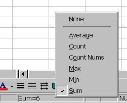 Choose the relevant option. For example, if I am interested in finding the maximum value in a particular range, I shall choose Max.
 3.4 SUBTOTAL() Function
In case there are nested totals, the SUM function can create havoc as there would be multiple totals. In such a situation one can consider the use of SUBTOTAL() function. This function avoids the cascading effect of the SUM function by recognizing the multilayered totaling feature. Accordingly, a subtotal function ignores the value of another subtotal function in the selected range of cells. The subtotal function is not restricted merely to the summation but can also be used for counts, etc. Accordingly, the SUBTOTAL() Function requires an additional argument which is the function number. The various function numbers and the action performed by them are tabulated below:
Function Number Action
1 AVERAGE
2 COUNT
3 COUNTA
4 MAX
5 MIN
6 PRODUCT
7 STDEV
8 STDEVP
9 SUM 10 VAR 11 VARP
3.5 SUMIF() Function
There might be situations wherein one wants to total only particular values within a list. In such a scenario, one can use the SUMIF() Function. This function evaluates the values for a specific condition and accordingly includes them for summation. The arguments for the SUMIF Function are:
Criteria Range: Criteria:
Sum Range: The range specifying the parameter or the condition The exact condition
The values to total
A cousin of SUMIF() Function is the COUNTIF() Function which counts the number of cells satisfying a particular criteria. In fact, the COUNTIF() Function can be combined with the Data Validation Feature to effectively stop the input of duplicate entries within a range of cells.
3.6 Sorting DataIn case a list of data is typed, one may need the data arranged in a particular fashion. For example, you may want your client details either alphabetically or based on the client codes. This is where sorting is useful and the same is very simple. Choose the relevant command from the Data Menu and the Sort Wizard takes you through the rest of the process. Remember, sorted data is always advantageous from three counts: firstly, it improves readability, secondly, it permits effective lookups and lastly, it lays down the foundation for data grouping and sub-totalling.
Sorting is a permanent process as compared to filtering which is a temporary processChoose any cell in the data range and Select Data -> Sort
Choose successive sort keys and sort order
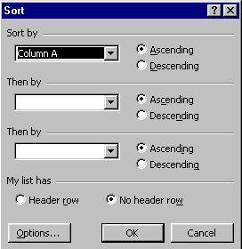
On a brief review of the above screen, one understands that the sort function permits sorting only upto three levels of data. If sorting is required for multiple levels of data, then one will have to use the sort function more than once. Sort first based on keys of least significance and move to keys of higher significance.
3.7 Sub-TotalsAt times, there is a need to not only have grand totals but also subtotals – would you not like to have group-wise outstanding as well as total outstanding? For this
Describe what you're looking for in as much detail as you'd like.
Our AI reads your request and finds the best matching books for you.
Popular searches:
Join 2.9 million readers and get unlimited free ebooks