2. DETERMINING THE REQUIRED QUANTITIES OF PARTS, COMPONENTS AND RAW MATERIALS. CALCULATING MANUFACTIRING/DELIVERY TIMES.___________________________ 10
2.1. CONDITIONAL ASSUMPTIONS _____________________________________10
2.2. CALCULATIONS AND ANALYSIS___________________________________10
2.3. RESULTS ________________________________________________________17
3. PRELIMINARY SCHEDULE _____________________________________ 19 3.1. IDENTIFICATION OF INITIAL SET OF LIMITATIONS __________________19 3.2. CRITICAL PATH ANALISYS ________________________________________20 3.3. DRAWING UP A PRELIMINARY SHEDULE ___________________________21 3.4. DETERMINING THE CRITICAL PATH COMPONENT___________________25 3.5. SUMMARY OF TIMES INCLUDED IN THE PRELIMINARY SCHEDULE___26
4. SCHEDULE OPTIMISATION ____________________________________ 271. DISCUSSION ON THE STRATEGY USED _________________________ 35 1.1. STRATEGY_______________________________________________________35 1.2. TACTICS _________________________________________________________36 1.3. TECHNIQUES_____________________________________________________36 1.4. POSITIVE EFFECTS OF THE ADOPTED TACTICS _____________________37 1.5. ADVANTAGES OF THE STRATEGY _________________________________38
2. APPLICABILITY OF THE TECHNIQUE FOR VARIOUS TYPES OF PRODUCTION AREAS_______________________________________ 394. LOADING STRATEGY RELATIVE TO CAPACITY (PROPOSAL)____ 46 4.1. BATCH SIZE______________________________________________________46 4.2. ANALYSIS OF STOCK INVENTORY _________________________________46 4.3. TIME BASED PRIORITY OF COMPONENT PARTS _____________________46 4.4. PRELIMINARY SCHEDULE_________________________________________47 4.5. RISK ANALYSIS __________________________________________________47 4.6. SCHEDULE OPTIMISATION ________________________________________48
Using the provided loading case study, make a schedule of the production load for the specified assemblies of components relative to the available production capacity. Estimate the earliest date of delivery ex-manufacturer’s warehouse for an order placed in the 20th week for 100 assemblies (product type A). Additionally, estimate the starting and final week for each individual subassembly and component and the date of ordering raw materials. Use both forward and backward load.
Key Words: Schedule; Loading; Forward Loading; Backward Loading; Critical Path Analysis; Critical Path Component; Finite LoadingINTRODUCTION
Operations and quality management involves the management of resources for the production of goods and services. This includes such functions as work force planning, inventory management, logistics management, production planning and control, resource allocation; and emphasises total quality management principles. Operations managers deal with people, materials, technology and deadlines (Halevi, 2001).
Loading indicates the specified time required to produce a single unit of the specified product in individual manufacturing facilities involved in the production of the product and further placement of orders to production departments, such that: an optimum utilisation of available resources is achieved; facilities overload is avoided; realistic dates of producing ordered quantities are defined; out-of balance production facilities are highlighted in order to take any corrective action as necessary to avoid this situation (Karmarkar, 1993).
Limit loading implies to load the work schedule of a specific production unit until the time corresponding to the specified capacity of this facility is reached. This particular method of load definition is used to determine the realistic dates of delivery of required component parts and products. It is assumed here that a limit capacity has already been defined for each individual production unit to be involved (Powell et all., 1995). Additionally, it is also assumed that loading information for each individual order is already available by the time the order is placed to the production department, as is the case being discussed here. The problem to be solved here is how to distribute this load information among different production units.
The two methods to accomplish this distribution are the Forward and backward loading. The forward loading begins with the present date and loads jobs forward in time. The processing time is accumulated against each work centre, assuming infinite or finite capacity. In this case, due dates may be exceeded if necessary. Since average waiting times are used in queues, the resulting job completion date is only an approximation of the date which might be calculated by more precise scheduling. The purpose of forward loading is to determine the approximate completion date of each job and, in the case of infinite capacity, the capacity required in each time period (Lyons, 2004). Backward loading begins with the due date for each job and loads the processing-time requirements against each work centre by proceeding backward in time. The capacity of work centres may be exceeded if necessary.
The purpose of backward loading is to calculate the capacity required in each work centre for each time period. As a result, it may be decided that capacity should be reallocated between work centres or that more total capacity should be made available through revised aggregate planning as suggested in Kats (2008). Due dates of jobs are always given for backward loading.
In current loading case study, a schedule of the production load for the specified assemblies of components relative to the available production capacity has been created. Estimations also on the earliest date of delivery ex-manufacturer’s warehouse for an order placed in the 20th week for 100 assemblies (product type A) have been processed. Additionally, the starting and final week for each individual sub-assembly and component and the date of ordering raw materials have been estimated, using both forward and backward loading.
In present case study, the load scheduling for the production of specified assemblies relevant to the available capacity had to go through the following stages: (a) Make an analysis of preliminary data (structural and quantitative interrelations between product A and its components) and visualisation of the product by means of presenting it in an exploded view; (b) Estimate and analyse times of delivery, manufacturing and assembly of raw materials, component parts and products along with the required quantities of each; (c) Determine the Critical Path Component (by synthesising initial limitations, performing Critical Path Analysis (Shapiro, 1993) and drawing up a preliminary schedule for a simplified set of conditions with the Forward Loading technique; (d) Carry out secondary loading for the production of the rest of the component parts on available free facilities applying the Backward Loading technique (Gamberi, 1998). Determine the high-risk areas taking actions to re-design and optimise the final real version; and (e) based on the schedule and inventory data, determine high-risk areas and suggest measures from a manager’s viewpoint.
When loading production departments manufacturing or assembling the specified component parts and assemblies we aimed at fitting the new order into the current production schedule while providing for the following: achieve the earliest possible realistic date of delivery ex-manufacturer’s warehouse of the order for 100 assemblies (product A) placed during week 20; achieve efficient loading of manufacturing facilities; ensure for the completion of current orders (without disturbing their specified delivery dates); reduce risks for order completion to a minimum and prevent their occurrence in current orders; avoid risks for orders placed at a later date but with earlier delivery times; guarantee for the interest of customers thus respecting the image of the company (Bobrowski, 1989).
The strategic aim has been to ensure the order was completed with the optimum load on production facilities and observing the delivery times and contractual terms agreed with the client. An integrated solution to the task, which actually comprised the system of interrelated sub-aims, would guarantee achieving not only the strategic aim but also bringing advantages to fortify marketing company achievements (Sarker, 1999).
The achievement of each strategic aim was accompanied by adopting specific tactics, accomplished in two stages: (a) Preparing a preliminary schedule of loading free facilities with the production of the new order using the Forward Loading technique. Extreme load was applied on the facilities since the utmost capacity of every facility involved in the process has already been identified and the loading information is already available for every order by the time it arrives in the production department. The purpose of this stage is to define the Critical Path Component. Loading was scheduled under several simplified preconditions: lack of any rejects, and failure-free operation. (b) Optimisation of the preliminary schedule by means of performing another loading applying the Backward Loading technique relative to the Critical Path Component (Desrosiers, 1995). Identifying the high-risk areas and reducing risks to a minimum by means of adopting appropriate measures.
ANALYSIS AND EXPLODING VIEW OF THE FINAL ASSEMBLYPerforming this type of analysis will help us clarify the structural and quantitative interrelations between assemblies and component parts comprising product A (Fredendall, 2010). Additionally, this will also help identify preliminary limitations in the time aspect such as, which assemblies can be assembled after a particular component part is manufactured.
LOADING CASE SCENARIOA manufacturer of the product A has received during the 20th week an order for 100 units of the specified product. Product A is an assembly made up of several individual components (see Table 1):
Table 1: Bill of Material for Assy.Part No Qty. Category B1 4 PP B2 4 PP B3 1 Assy B4 1 Assy
Man. Code Bought out Bought out
Made In Made In On the other hand, these components comprise a number of sub-assemblies and individual parts and Tables 2, 3 and 4 show their quantities and category characteristics:
Table 2: Bill of Material for Assy. 3 Part No Qty. Category
C1 1 Assy C2 2 PP C3 1 PP
Man. Code Made In Made In
Bought outTable 3: Bill of Material for Assy. 4
Part No Qty. Category E1 1 PP E2 1 PP B1 4 PP B2 4 PP
Man. Code Made In Made In
Bought out Bought outTable 4: Bill of Material for Assy. C1
Part No Qty. Category C2 2 PP D1 1 PP
Man. Code Made In Made In
Table 5 shows the current inventory of component parts and raw materials at the moment of placement of the order:Table 5: Current Stock Position – Week 20
Part No Available stock Ordered
B1 200 Nil B2 1000 Nil
C2 340 Nil C3 200 Nil
D1 30 Nil E2 80 Nil
RM1 600 m Nil RM2 60 m Nil
RM3 120 m Nil
Table 6 systemises information on production department areas involved in the assembly process for the relevant sub-assemblies along with process times required for: withdrawal from store, assembly, inspection and transfer.
Table 6: Assemblies Manufacturing InformationPart Dept. Stores Assembly Time Inspection / No Code Storage (each) Transfer Time Times
A FA 1 week 0.28 h 2 days B3 SA1 2 days 0.56 h 2 days B4 SA2 2 days 0.37 h 2 days C1 SA3 2 days 0.70 h 2 days
Table 7 shows manufacturing information relating to made in component parts and Table 8 shows information for bought out component parts and raw materials.
Table 7: Piece Parts Made InBatch Part Dept. Adjustment Operation No Code Time Time
C2 D1 4 h 70 h D1 T2 2 h 2 h E1 G1 8 h 25 h E2 H2 6 h 30 h
Inspection Matl. Raw Raw & transfer E.B.Q. Matl. Matl. Time Code /E.B.Q.
1 day 1000 RM2 140 m 2 days 500 RM3 130 m 2 days 250 RM2 120 m 1 day 300 RM1 150 m
Table 8: Piece Part & Row Material Bought OutPart No Delivery Time Economic Order Quantity (E.O.Q) B1 2 weeks 3000 B2 2 weeks 3000 C3 4 weeks 500
RM1 8 weeks 1000 m RM2 6 weeks 2000 m RM3 4 weeks 500 m
Table 9 shows the workload at the moment of receipt of the order for 100 pcs. of type A product:Table 9: Current Load – Week 20
Dept. Cap. O/D Wk Wk Wk Wk Wk Wk Wk Wk Wk Wk Wk Wk Wk Wk Wk Wk Wk /Hrs/ /Hrs/ No No No No No No No No No No No No No No No No No 20 21 22 23 24 25 26 27 28 29 30 31 32 33 34 35 36 FA 40 4 40 40 40 40 38 38 40 40 40 40 40 40 40 40 39 38 0
SA1 40 - 40 40 40 40 40 40 40 40 40 40 40 40 40 38 0 0 0
SA2 40 12 40 40 40 40 40 35 36 37 40 40 35 28 31 3 0 0 0 SA3 40 16 40 40 40 40 40 40 32 36 34 32 30 20 10 5 5 0 0
D1 40 8 40 40 40 40 32 34 40 30 20 20 15 10 8 0 0 0 0 T2 40 10 40 40 40 40 35 30 28 17 17 15 10 9 7 0 0 0 0
G1 40 11 40 40 40 40 35 34 40 20 15 15 12 10 0 0 0 0 0 H2 40 15 40 40 40 40 32 36 39 38 10 10 10 9 0 0 0 0 0
Key;
Dept = Department; Cap. = Capacity; O/D = Overdue Hours; Wk = Week; PP = part; = product; RM = Raw Materials; FA – Final Assembly; SA = Sub-Assembly; E.B.Q. = Economic Batch Quantity; E.O.Q. = Economic Order Quantity.
Operations and Quality Management involves the management of resources for the production of goods and services. This includes such functions as work force planning, inventory management, logistics management, production planning and control, resource allocation; and emphasises total quality management principles. Operations managers deal with people, materials, technology and deadlines.
Loading indicates the specified time required to produce a single unit of the specified product in individual manufacturing facilities involved in the production of the product and further placement of orders to production departments, such that:
an optimum utilisation of available resources is achieved;
facilities overload is avoided;
realistic dates of producing ordered quantities are defined;
out-of balance production facilities are highlighted (in order to take any corrective action as necessary to avoid this situation).
Limit loading means to load the work schedule of a specific production unit until the time corresponding to the specified capacity of this facility is reached. This particular method of load definition is used to determine the realistic dates of delivery of required component parts and products. It is assumed here that a limit capacity has already been defined for each individual production unit to be involved. Additionally, it is also assumed that loading information for each individual order is already available by the time the order is placed to the production department, as is the case being discussed here. The problem to be solved here is how to distribute this load information among different production units. The two methods to accomplish this are:
Forward loading . Begins with the present date and loads jobs forward in time. The processing time is accumulated against each work centre, assuming infinite or finite capacity. In this case, due dates may be exceeded if necessary. Since average waiting times are used in queues, the resulting job completion date is only an approximation of the date which might be calculated by more precise scheduling. The purpose of forward loading is to determine the approximate completion date of each job and, in the case of infinite capacity, the capacity required in each time period.
Backward loading . Begins with the due date for each job and loads the processing-time requirements against each work centre by proceeding backward in time. The capacity of work centres may be exceeded if necessary. The purpose of backward loading is to calculate the capacity required in each work centre for each time period. As a result, it may be decided that capacity should be reallocated between work centres or that more total capacity should be made available through revised aggregate planning. Due dates of jobs are always given for backward loading.
METHODOLOGYIn the case study provided, the load scheduling for the production of specified assemblies relevant to the available capacity will go through the following stages:
Make an analysis of preliminary data (structural and quantitative interrelations between product A and its constituent components) and visualisation of the product by means of presenting it in an exploded view;
Estimate and analyse times of delivery, manufacturing and assembly of raw materials, component parts and products along with the required quantities of each;
Determine the Critical Path Component by means of synthesising initial limitations, perform Critical Path Analysis and draw up a preliminary schedule for a simplified set of conditions and applying the Forward Loading technique;
Carry out secondary loading for the production of the rest of the component parts on available free facilities applying the Backward Loading technique. Determine the high-risk areas and take appropriate actions to re-design and optimise the final real version.
1. ANALYSIS AND EXPLODING VIEW OF FINAL ASSEMBLYPerforming this type of analysis will help us clarify the structural and quantitative interrelations between assemblies and component parts comprising product A. Additionally, this will also help us identify some preliminary limitations in the time aspect, such as, for example, which assemblies can be assembled after a particular component part is manufactured.
The final assembly comprises the following component parts: B1, B2, B3, B4, C1, C2, C3, D1, E1, E2.Of them: B1, B2 and C3 are bought out components;
C2, D1, E1 and E2 are made in by the manufacturer’s production departments;B3, B4 and C1 are sub-assemblies, which in turn need to be assembled; Raw materials RM1, RM2 and RM3 are bought out and used for manufacturing made in component parts (C2, D1, E1 and E2).
It is important to note here that identical quantities (4 pcs.) of parts B1 and B2
are used for both the finished product A and for sub-assembly B4 (see Table 1
and Table 3). Similarly, component C2 is used both in assembly B3 and in its sub-assembly C1 (see Table 2 and Table 4). This is important to be kept in mind, since, depending on the availability of free production facilities, the assembly of sub-assemblies can start at an earlier date if sufficient stock inventory of these components is available and this will have an influence on the order completion time.
Above analysis and Tables 1, 2, 3, 4 and 7 allow us to present product A in the following “exploded” view:
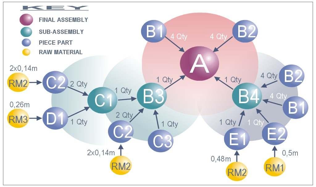
It could also be presented for a more detailed and analitical view in the following way:
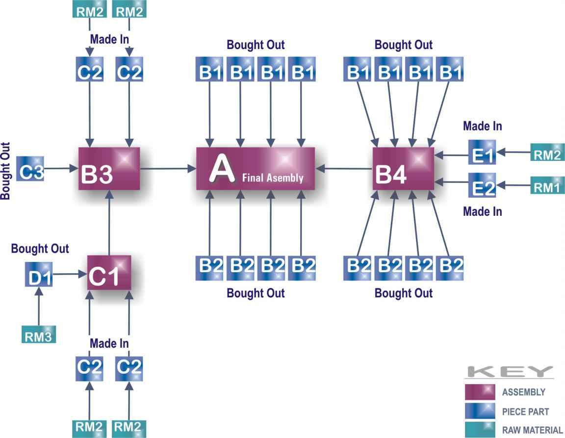 Fig. 1 Exploded View of the Final Assembly A
 2. DETERMINING THE REQUIRED QUANTITIES OF PARTS, COMPONENTS AND RAW MATERIALS. CALCULATING MANUFACTIRING/DELIVERY TIMES.
The following parameters need to be calculated for product A and each of its component parts in order to be able to make out the schedule for the specific order of 100 units of product A and draw up the work load for the available capacities:
The required quantity of component parts or materials, keeping in mind the available stock inventory at the time of receipt of the specific order; The time for ordering, delivering, withdrawal from store, manufacturing/assembly, inspection and handling.Thus, total times for product A and for each of its individual component parts will be estimated and will eventually be used to fill up available free capacity.
2.1. CONDITIONAL ASSUMPTIONS The process of drawing up the preliminary simplified schedule will be accompanied by the following conditional assumptions:
One working week is 5 days and one working day is 8 hours; No damaged or out-of-spec component parts, products or raw materials are present in the production process;
No equipment failures will be registered in the production, which will in turn allow us to work with minimum order quantities.
Stock inventory data is accurate thus avoiding the need for out-ofschedule deliveries.
In other words, a preliminary schedule will be drawn up for an ideal set of conditions and this will eventually be modified and optimised based on the risk analysis and the adoption of some new managing solutions to make up the real production schedule.
2.2. CALCULATIONS AND ANALYSISCalculations and analysis of times for manufacturing/delivery of component parts, products and raw materials as well as the required quantities of each, is as follows:
Product :This is the finished product and 100 units of this product have to be assembled. Store withdrawal time is 1week (Table 6) or 40 h.
Time required to assemble a single unit of product A is 0.28h (Table 6) or
100 x 0.28h = 28h for 100 units of product.
Therefore, the total time TA required to assemble, withdraw from store and handle 100 units of product A will then be:
TA = 40h + 100x0.28h + 16h = 84h
Component B1:
This is a bought out component and 8 pcs. of component B1 are used for one unit of product A. 4pcs. of them are used directly in the final assembly stage (Table 1) and another 4 pcs. are used for the sub-assembly B4 (Table 3). The total quantity of components B1 required for the entire order of 100 units of product A is 800 pcs. Current stock inventory indicates 200 pcs. of component B1 are available in store (Table 5). No order for a new batch of components B1 is placed during the 20th week. Therefore, another 600pcs of component B1 will have to be ordered in order to have sufficient quantity to assemble 100 units of product A. But Table 8 shows that the Economic Order Quantity (E.O.Q) is 3000 pcs. Delivery time for component 1 (TB1) is 2 weeks or 80h (Table. 8).
TB1 = 80hDelivery time is the same for both a quantity of 600 pcs and for 3000 pcs of component B1. A better management solution would be to place an order for 3000 pcs of B1 since this component is used in large quantities for assembling product A and it would be wise to have some inventory left in stock after the order for 100 pcs of product A is completed.
Component B2:This is again a bought out component and 8 pcs. of component B2 are used for one unit of product A. 4pcs. of them are used directly in the final assembly stage (Table 1) and another 4 pcs. are used for sub-assembly B4 (Table 3). The total quantity of components B2 required for the entire order of 100 units of product A is 800 pcs. Current stock inventory (Table 5) indicates 1000 pcs. of component B2 are available in store. Therefore, this will provide for the assembly of 100 units of product A and no additional quantity of component B2 needs to be ordered. Moreover, 200 pcs B2 will still be left in stock after withdrawal of 800 of them for assembly. Therefore, we do not need to estimate delivery time for component 2.
TB2 = 0hComponent B3:
This is assembled in production department SA1 and 1 pc. B3 is used per each product A. Therefore, 100 pcs. of B3 are required for an order of 100 units of product A. No stock inventory of B3 is currently available (Table 5). Subassembly B3 comprises product C1 and parts C2 and C3. Therefore, we need to assemble 100 pcs. of B3 in order to have sufficient quantity for the ordered 100 pcs. of product A.
The time of withdrawal of B3 from stock is 2 days (Table 6) or 16h. 1 piece of 3 is assembled for 0,56h (Table 6) or 100 x 0.56h = 56h for 100pcs.Inspection and handling time is 2 days (Table 6) or 16h.
The total time TB3 required to assemble, withdraw and move 100 pcs. of B3 will be:
TB3 = 16h + 100x0.56h +16h = 88h
Product B4:
This is assembled in production department SA2 and 1pc. B4 is used per each product A. Therefore, 100 pcs. of B4 are required for an order of 100 units of product A. No stock inventory of B4 is currently available (Table 5). Subassembly B4 comprises components B1, B2, E1 and E2. Therefore, we need to assemble 100 pcs. of B4 in order to have sufficient quantity for the ordered 100 pcs. of product A.
The time of withdrawal of B4 from stock is 2 days (Table 6) or 16h. 1 piece of 4 is assembled for 0,37h (Table 6) or 100 x 0.37h = 37h for 100pcs.Inspection and handling time is 2 days (Table 6) or 16h.
The total time TB4 required to assemble, withdraw and move 100 pcs. of B4 will be:
TB4 = 16h + 100x0.37h +16h = 69h
Product !1:
This is assembled in production department SA3 and it is a constituent part of product B3 (Table 2) and 1 pc. C1 is used per each B3.C1 is assembled from C2 and D1 (Table 4). 100 pcs. of B3 and hence, 100 pcs. C1 are required for an order of 100 units of product A. No stock inventory of C1 is currently available (Table 5). Therefore, we need to assemble 100 pcs. of C1 in order to have sufficient quantity for the ordered 100 pcs. of product A.
The time of withdrawal of C1 from stock is 2 days (Table 6) or 16h. 1 piece of 3 is assembled for 0,7h (Table 6) or 100 x 0.7h = 70h for 100pcs.Inspection and handling time is 2

Reads:
39
Pages:
62
Published:
Jul 2025
Uncover the wonders of STEM with this 400 Fun Facts book! From mind-bending physics to the mysteries of the universe, dive into an engaging collection that sp...
Formats: PDF, Epub, Kindle, TXT

Reads:
445
Pages:
1608
Published:
Dec 2024
"Scientific Evidence for Reincarnation, NDEs and Karma with Personal Stories" is a free book that shows you the truth about reincarnation. It contains a lot o...
Formats: PDF, Epub, Kindle, TXT

Reads:
7
Pages:
38
Published:
Dec 2024
Trabajo sobre la toponimia actual en el término municipal de San Fernando (Cádiz)
Formats: PDF, Epub, Kindle, TXT

Reads:
205
Pages:
166
Published:
Jun 2023
Embark on a cosmic journey as we delve into the mysteries of the universe and the frontiers of space. From the Big Bang and black holes to exoplanets and the ...
Formats: PDF, Epub, Kindle, TXT
Describe what you're looking for in as much detail as you'd like.
Our AI reads your request and finds the best matching books for you.
Popular searches:
Join 2.9 million readers and get unlimited free ebooks